TLG Catalog - Stable
  • Stable
    • Dev
  1. Tables
  2. Lab Results
  3. LBT13
  • Introduction

  • Tables
    • ADA
      • ADAT01
      • ADAT02
      • ADAT03
      • ADAT04A
      • ADAT04B
    • Adverse Events
      • AET01
      • AET01_AESI
      • AET02
      • AET02_SMQ
      • AET03
      • AET04
      • AET04_PI
      • AET05
      • AET05_ALL
      • AET06
      • AET06_SMQ
      • AET07
      • AET09
      • AET09_SMQ
      • AET10
    • Concomitant Medications
      • CMT01
      • CMT01A
      • CMT01B
      • CMT02_PT
    • Deaths
      • DTHT01
    • Demography
      • DMT01
    • Disclosures
      • DISCLOSUREST01
      • EUDRAT01
      • EUDRAT02
    • Disposition
      • DST01
      • PDT01
      • PDT02
    • ECG
      • EGT01
      • EGT02
      • EGT03
      • EGT04
      • EGT05_QTCAT
    • Efficacy
      • AOVT01
      • AOVT02
      • AOVT03
      • CFBT01
      • CMHT01
      • COXT01
      • COXT02
      • DORT01
      • LGRT02
      • MMRMT01
      • ONCT05
      • RATET01
      • RBMIT01
      • RSPT01
      • TTET01
    • Exposure
      • EXT01
    • Lab Results
      • LBT01
      • LBT02
      • LBT03
      • LBT04
      • LBT05
      • LBT06
      • LBT07
      • LBT08
      • LBT09
      • LBT10
      • LBT10_BL
      • LBT11
      • LBT11_BL
      • LBT12
      • LBT12_BL
      • LBT13
      • LBT14
      • LBT15
    • Medical History
      • MHT01
    • Pharmacokinetic
      • PKCT01
      • PKPT02
      • PKPT03
      • PKPT04
      • PKPT05
      • PKPT06
      • PKPT07
      • PKPT08
      • PKPT11
    • Risk Management Plan
      • RMPT01
      • RMPT03
      • RMPT04
      • RMPT05
      • RMPT06
    • Safety
      • ENTXX
    • Vital Signs
      • VST01
      • VST02
  • Listings
    • ADA
      • ADAL02
    • Adverse Events
      • AEL01
      • AEL01_NOLLT
      • AEL02
      • AEL02_ED
      • AEL03
      • AEL04
    • Concomitant Medications
      • CML01
      • CML02A_GL
      • CML02B_GL
    • Development Safety Update Report
      • DSUR4
    • Disposition
      • DSL01
      • DSL02
    • ECG
      • EGL01
    • Efficacy
      • ONCL01
    • Exposure
      • EXL01
    • Lab Results
      • LBL01
      • LBL01_RLS
      • LBL02A
      • LBL02A_RLS
      • LBL02B
    • Medical History
      • MHL01
    • Pharmacokinetic
      • ADAL01
      • PKCL01
      • PKCL02
      • PKPL01
      • PKPL02
      • PKPL04
    • Vital Signs
      • VSL01
  • Graphs
    • Efficacy
      • FSTG01
      • FSTG02
      • KMG01
      • MMRMG01
      • MMRMG02
    • Other
      • BRG01
      • BWG01
      • CIG01
      • IPPG01
      • LTG01
      • MNG01
    • Pharmacokinetic
      • PKCG01
      • PKCG02
      • PKCG03
      • PKPG01
      • PKPG02
      • PKPG03
      • PKPG04
      • PKPG06

  • Appendix
    • Reproducibility

  • Index

On this page

  • Output
  • teal App
  • Reproducibility
    • Timestamp
    • Session Info
    • .lock file
  • Edit this page
  • Report an issue
  1. Tables
  2. Lab Results
  3. LBT13

LBT13

NCI CTCAE Grade Laboratory Abnormalities by Visit and Baseline Grade


Output

  • Standard Table (Low)
  • Standard Table (High)
  • Table Without Patients with
    Missing Baseline (Low)
  • Table with Missing Baseline
    Considered as Grade 0 (High)
  • Table with Fill-In
    of Grades (High)
  • Data Setup

Note that the worst laboratory flag (below WGRLOVFL) must be selected appropriately to match the direction of abnormality (here Low). New grouping variables ATOXGR_GP and BTOXGR_GP are created to display the correct output.

  • Preview
  • Try this using WebR
Code
adlb_f <- adlb %>% filter(WGRLOVFL == "Y")

# Please note the step below can be skipped if you are using DTYPE PHANTOM
adlb_out <- adsl_f %>%
  h_adsl_adlb_merge_using_worst_flag(
    adlb_f,
    worst_flag = c("WGRLOVFL" = "Y"),
    by_visit = TRUE,
    no_fillin_visits = c("SCREENING", "BASELINE", "UNSCHEDULED")
  )

# Create new grouping variables ATOXGR_GP, BTOXGR_GP
adlb_out <- adlb_out %>%
  mutate(
    ATOXGR_GP = case_when(
      ATOXGR %in% c(0, 1, 2, 3, 4) ~ "Not Low",
      ATOXGR == -1 ~ "1",
      ATOXGR == -2 ~ "2",
      ATOXGR == -3 ~ "3",
      ATOXGR == -4 ~ "4",
      ATOXGR == "<Missing>" ~ "Missing"
    )
  ) %>%
  mutate(
    BTOXGR_GP = case_when(
      BTOXGR %in% c(0, 1, 2, 3, 4) ~ "Not Low",
      BTOXGR == -1 ~ "1",
      BTOXGR == -2 ~ "2",
      BTOXGR == -3 ~ "3",
      BTOXGR == -4 ~ "4",
      BTOXGR == "<Missing>" ~ "Missing"
    )
  )

adlb_out <- adlb_out %>% mutate(
  AVISIT = forcats::fct_reorder(AVISIT, AVISITN),
  ATOXGR_GP = factor(ATOXGR_GP, levels = c("Not Low", "1", "2", "3", "4", "Missing")),
  BTOXGR_GP = factor(BTOXGR_GP, levels = c("Not Low", "1", "2", "3", "4", "Missing"))
)

adlb_out <- adlb_out %>%
  var_relabel(
    PARAMCD = "Parameter Code",
    AVISIT = "Visit",
    ATOXGR_GP = "NCI CTCAE Grade at Visit",
    BTOXGR_GP = "Baseline NCI CTCAE Grade"
  )

result <- basic_table(show_colcounts = TRUE) %>%
  split_cols_by("ACTARM") %>%
  split_rows_by(
    "PARAMCD",
    split_fun = drop_split_levels, label_pos = "topleft", split_label = obj_label(adlb_out$PARAMCD)
  ) %>%
  split_rows_by(
    "AVISIT",
    split_fun = drop_split_levels, label_pos = "topleft", split_label = obj_label(adlb_out$AVISIT)
  ) %>%
  split_rows_by(
    "ATOXGR_GP",
    split_fun = drop_split_levels, label_pos = "topleft", split_label = obj_label(adlb_out$ATOXGR_GP)
  ) %>%
  summarize_num_patients(var = "USUBJID", .stats = c("unique_count")) %>%
  count_occurrences("BTOXGR_GP", denom = "n", drop = TRUE) %>%
  append_varlabels(adlb_out, "BTOXGR_GP", indent = 3L) %>%
  build_table(df = adlb_out, alt_counts_df = adsl_f)

result
Parameter Code                                                             
  Visit                                                                    
    NCI CTCAE Grade at Visit      A: Drug X    B: Placebo    C: Combination
      Baseline NCI CTCAE Grade     (N=134)       (N=134)        (N=132)    
———————————————————————————————————————————————————————————————————————————
CRP                                                                        
  WEEK 1 DAY 8                                                             
    Not Low (n)                      116           110            101      
      Not Low                    103 (88.8%)   91 (82.7%)      88 (87.1%)  
      1                           3 (2.6%)      5 (4.5%)        6 (5.9%)   
      2                           4 (3.4%)      9 (8.2%)        2 (2.0%)   
      3                           3 (2.6%)      4 (3.6%)        4 (4.0%)   
      4                           3 (2.6%)      1 (0.9%)        1 (1.0%)   
    1 (n)                             4             7              5       
      Not Low                     3 (75.0%)     7 (100%)       4 (80.0%)   
      3                           1 (25.0%)         0          1 (20.0%)   
    2 (n)                             5             6              11      
      Not Low                     5 (100%)      5 (83.3%)      8 (72.7%)   
      1                               0             0           1 (9.1%)   
      3                               0             0          2 (18.2%)   
      4                               0         1 (16.7%)          0       
    3 (n)                             6             8              5       
      Not Low                     6 (100%)      7 (87.5%)       5 (100%)   
      3                               0         1 (12.5%)          0       
    4 (n)                             3             3              10      
      Not Low                     2 (66.7%)     3 (100%)       7 (70.0%)   
      1                               0             0          2 (20.0%)   
      2                           1 (33.3%)         0              0       
      4                               0             0          1 (10.0%)   
  WEEK 2 DAY 15                                                            
    Not Low (n)                      106           111            116      
      Not Low                    93 (87.7%)    93 (83.8%)     100 (86.2%)  
      1                           3 (2.8%)      4 (3.6%)        8 (6.9%)   
      2                           5 (4.7%)      7 (6.3%)        2 (1.7%)   
      3                           2 (1.9%)      5 (4.5%)        6 (5.2%)   
      4                           3 (2.8%)      2 (1.8%)           0       
    1 (n)                            15             9              2       
      Not Low                    13 (86.7%)     8 (88.9%)      1 (50.0%)   
      2                               0         1 (11.1%)          0       
      3                           2 (13.3%)         0              0       
      4                               0             0          1 (50.0%)   
    2 (n)                             3             3              6       
      Not Low                     3 (100%)      3 (100%)       4 (66.7%)   
      1                               0             0          1 (16.7%)   
      3                               0             0          1 (16.7%)   
    3 (n)                             7             7              6       
      Not Low                     7 (100%)      6 (85.7%)      5 (83.3%)   
      2                               0         1 (14.3%)          0       
      4                               0             0          1 (16.7%)   
    4 (n)                             3             4              2       
      Not Low                     3 (100%)      3 (75.0%)       2 (100%)   
      1                               0         1 (25.0%)          0       
  WEEK 3 DAY 22                                                            
    Not Low (n)                      119           110            114      
      Not Low                    104 (87.4%)   92 (83.6%)      94 (82.5%)  
      1                           3 (2.5%)      4 (3.6%)        9 (7.9%)   
      2                           5 (4.2%)      7 (6.4%)        2 (1.8%)   
      3                           4 (3.4%)      5 (4.5%)        7 (6.1%)   
      4                           3 (2.5%)      2 (1.8%)        2 (1.8%)   
    1 (n)                             9             9              6       
      Not Low                     9 (100%)      7 (77.8%)       6 (100%)   
      2                               0         2 (22.2%)          0       
    2 (n)                             1             7              3       
      Not Low                     1 (100%)      6 (85.7%)       3 (100%)   
      1                               0         1 (14.3%)          0       
    3 (n)                             4             5              4       
      Not Low                     4 (100%)      5 (100%)        4 (100%)   
    4 (n)                             1             3              5       
      Not Low                     1 (100%)      3 (100%)        5 (100%)   
  WEEK 4 DAY 29                                                            
    Not Low (n)                      101           119            111      
      Not Low                    89 (88.1%)    100 (84.0%)     96 (86.5%)  
      1                           3 (3.0%)      4 (3.4%)        6 (5.4%)   
      2                           4 (4.0%)      8 (6.7%)        1 (0.9%)   
      3                           2 (2.0%)      5 (4.2%)        6 (5.4%)   
      4                           3 (3.0%)      2 (1.7%)        2 (1.8%)   
    1 (n)                            10             5              6       
      Not Low                     9 (90.0%)     5 (100%)       5 (83.3%)   
      1                               0             0          1 (16.7%)   
      2                           1 (10.0%)         0              0       
    2 (n)                            13             4              6       
      Not Low                     13 (100%)     3 (75.0%)      5 (83.3%)   
      1                               0             0          1 (16.7%)   
      2                               0         1 (25.0%)          0       
    3 (n)                             8             2              6       
      Not Low                     6 (75.0%)     1 (50.0%)      5 (83.3%)   
      1                               0         1 (50.0%)          0       
      2                               0             0          1 (16.7%)   
      3                           2 (25.0%)         0              0       
    4 (n)                             2             4              3       
      Not Low                     2 (100%)      4 (100%)       1 (33.3%)   
      1                               0             0          1 (33.3%)   
      3                               0             0          1 (33.3%)   
  WEEK 5 DAY 36                                                            
    Not Low (n)                      115           112            111      
      Not Low                    102 (88.7%)   94 (83.9%)      96 (86.5%)  
      1                           2 (1.7%)      4 (3.6%)        6 (5.4%)   
      2                           5 (4.3%)      7 (6.2%)        2 (1.8%)   
      3                           3 (2.6%)      5 (4.5%)        5 (4.5%)   
      4                           3 (2.6%)      2 (1.8%)        2 (1.8%)   
    1 (n)                             5             7              6       
      Not Low                     5 (100%)      4 (57.1%)      5 (83.3%)   
      1                               0         1 (14.3%)      1 (16.7%)   
      2                               0         2 (28.6%)          0       
    2 (n)                             5            11              6       
      Not Low                     5 (100%)      11 (100%)       6 (100%)   
    3 (n)                             8             2              7       
      Not Low                     6 (75.0%)     2 (100%)       4 (57.1%)   
      1                           1 (12.5%)         0          1 (14.3%)   
      3                           1 (12.5%)         0          2 (28.6%)   
    4 (n)                             1             2              2       
      Not Low                     1 (100%)      2 (100%)       1 (50.0%)   
      1                               0             0          1 (50.0%)   
Experimental use!

WebR is a tool allowing you to run R code in the web browser. Modify the code below and click run to see the results. Alternatively, copy the code and click here to open WebR in a new tab.

Note that the worst laboratory flag (below WGRHIVFL) must be selected appropriately to match the direction of abnormality (here High). New grouping variables ATOXGR_GP and BTOXGR_GP are created to display the correct output.

  • Preview
  • Try this using WebR
Code
adlb_f <- adlb %>% filter(WGRHIVFL == "Y")

# Please note the step below can be skipped if you are using DTYPE PHANTOM
adlb_out <- adsl_f %>%
  h_adsl_adlb_merge_using_worst_flag(
    adlb_f,
    worst_flag = c("WGRHIVFL" = "Y"),
    by_visit = TRUE,
    no_fillin_visits = c("SCREENING", "BASELINE", "UNSCHEDULED")
  )

# Create new grouping variables ATOXGR_GP, BTOXGR_GP
adlb_out <- adlb_out %>%
  mutate(
    ATOXGR_GP = case_when(
      ATOXGR %in% c(0, -1, -2, -3, -4) ~ "Not High",
      ATOXGR == 1 ~ "1",
      ATOXGR == 2 ~ "2",
      ATOXGR == 3 ~ "3",
      ATOXGR == 4 ~ "4",
      ATOXGR == "<Missing>" ~ "Missing"
    )
  ) %>%
  mutate(
    BTOXGR_GP = case_when(
      BTOXGR %in% c(0, -1, -2, -3, -4) ~ "Not High",
      BTOXGR == 1 ~ "1",
      BTOXGR == 2 ~ "2",
      BTOXGR == 3 ~ "3",
      BTOXGR == 4 ~ "4",
      BTOXGR == "<Missing>" ~ "Missing"
    )
  )

adlb_out <- adlb_out %>% mutate(
  AVISIT = forcats::fct_reorder(AVISIT, AVISITN),
  ATOXGR_GP = factor(ATOXGR_GP, levels = c("Not High", "1", "2", "3", "4", "Missing")),
  BTOXGR_GP = factor(BTOXGR_GP, levels = c("Not High", "1", "2", "3", "4", "Missing"))
)

adlb_out <- adlb_out %>%
  var_relabel(
    PARAMCD = "Parameter Code",
    AVISIT = "Visit",
    ATOXGR_GP = "NCI CTCAE Grade at Visit",
    BTOXGR_GP = "Baseline NCI CTCAE Grade"
  )

result <- basic_table(show_colcounts = TRUE) %>%
  split_cols_by("ACTARM") %>%
  split_rows_by(
    "PARAMCD",
    split_fun = drop_split_levels, label_pos = "topleft", split_label = obj_label(adlb_out$PARAMCD)
  ) %>%
  split_rows_by(
    "AVISIT",
    split_fun = drop_split_levels, label_pos = "topleft", split_label = obj_label(adlb_out$AVISIT)
  ) %>%
  split_rows_by(
    "ATOXGR_GP",
    split_fun = drop_split_levels, label_pos = "topleft", split_label = obj_label(adlb_out$ATOXGR_GP)
  ) %>%
  summarize_num_patients(var = "USUBJID", .stats = c("unique_count")) %>%
  count_occurrences("BTOXGR_GP", denom = "n", drop = TRUE) %>%
  append_varlabels(adlb_out, "BTOXGR_GP", indent = 3L) %>%
  build_table(df = adlb_out, alt_counts_df = adsl_f)

result
Parameter Code                                                            
  Visit                                                                   
    NCI CTCAE Grade at Visit     A: Drug X    B: Placebo    C: Combination
      Baseline NCI CTCAE Grade    (N=134)       (N=134)        (N=132)    
——————————————————————————————————————————————————————————————————————————
CRP                                                                       
  WEEK 1 DAY 8                                                            
    Not High (n)                    111           110            112      
      Not High                   93 (83.8%)   92 (83.6%)      98 (87.5%)  
      1                           8 (7.2%)     7 (6.4%)        5 (4.5%)   
      2                           2 (1.8%)     6 (5.5%)        7 (6.2%)   
      3                           6 (5.4%)     3 (2.7%)        2 (1.8%)   
      4                           2 (1.8%)     2 (1.8%)           0       
    1 (n)                            8            11              6       
      Not High                   7 (87.5%)     11 (100%)      5 (83.3%)   
      3                          1 (12.5%)         0          1 (16.7%)   
    2 (n)                            6             4              5       
      Not High                    6 (100%)     1 (25.0%)      4 (80.0%)   
      1                              0         3 (75.0%)      1 (20.0%)   
    3 (n)                            8             3              4       
      Not High                   7 (87.5%)     3 (100%)        4 (100%)   
      4                          1 (12.5%)         0              0       
    4 (n)                            1             6              5       
      Not High                    1 (100%)     5 (83.3%)      4 (80.0%)   
      1                              0             0          1 (20.0%)   
      3                              0         1 (16.7%)          0       
  WEEK 2 DAY 15                                                           
    Not High (n)                    117           113            113      
      Not High                   99 (84.6%)   95 (84.1%)     100 (88.5%)  
      1                           7 (6.0%)     6 (5.3%)        4 (3.5%)   
      2                           2 (1.7%)     6 (5.3%)        6 (5.3%)   
      3                           6 (5.1%)     4 (3.5%)        3 (2.7%)   
      4                           3 (2.6%)     2 (1.8%)           0       
    1 (n)                            6             9              7       
      Not High                   5 (83.3%)     8 (88.9%)      6 (85.7%)   
      1                              0         1 (11.1%)          0       
      2                              0             0          1 (14.3%)   
      3                          1 (16.7%)         0              0       
    2 (n)                            4             4              6       
      Not High                    4 (100%)     4 (100%)       3 (50.0%)   
      1                              0             0          3 (50.0%)   
    3 (n)                            5             3              5       
      Not High                   4 (80.0%)     2 (66.7%)       5 (100%)   
      1                          1 (20.0%)     1 (33.3%)          0       
    4 (n)                            2             5              1       
      Not High                    2 (100%)     3 (60.0%)       1 (100%)   
      1                              0         2 (40.0%)          0       
  WEEK 3 DAY 22                                                           
    Not High (n)                    110           111            114      
      Not High                   92 (83.6%)   94 (84.7%)      98 (86.0%)  
      1                           8 (7.3%)     9 (8.1%)        7 (6.1%)   
      2                           2 (1.8%)     5 (4.5%)        6 (5.3%)   
      3                           5 (4.5%)     2 (1.8%)        3 (2.6%)   
      4                           3 (2.7%)     1 (0.9%)           0       
    1 (n)                            7             8              7       
      Not High                    7 (100%)     5 (62.5%)      6 (85.7%)   
      1                              0         1 (12.5%)          0       
      2                              0         1 (12.5%)      1 (14.3%)   
      3                              0         1 (12.5%)          0       
    2 (n)                            9             7              5       
      Not High                    9 (100%)     6 (85.7%)       5 (100%)   
      3                              0         1 (14.3%)          0       
    3 (n)                            6             3              4       
      Not High                   5 (83.3%)     2 (66.7%)       4 (100%)   
      3                          1 (16.7%)         0              0       
      4                              0         1 (33.3%)          0       
    4 (n)                            2             5              2       
      Not High                   1 (50.0%)     5 (100%)        2 (100%)   
      3                          1 (50.0%)         0              0       
  WEEK 4 DAY 29                                                           
    Not High (n)                    115           117            113      
      Not High                   97 (84.3%)   101 (86.3%)     99 (87.6%)  
      1                           8 (7.0%)     7 (6.0%)        6 (5.3%)   
      2                           2 (1.7%)     6 (5.1%)        5 (4.4%)   
      3                           7 (6.1%)     3 (2.6%)        3 (2.7%)   
      4                           1 (0.9%)         0              0       
    1 (n)                            4             3              11      
      Not High                    4 (100%)     2 (66.7%)      10 (90.9%)  
      2                              0             0           1 (9.1%)   
      4                              0         1 (33.3%)          0       
    2 (n)                            6             4              2       
      Not High                    6 (100%)     3 (75.0%)       2 (100%)   
      1                              0         1 (25.0%)          0       
    3 (n)                            6             7              4       
      Not High                   5 (83.3%)     4 (57.1%)       4 (100%)   
      1                              0         1 (14.3%)          0       
      3                              0         1 (14.3%)          0       
      4                          1 (16.7%)     1 (14.3%)          0       
    4 (n)                            3             3              2       
      Not High                   2 (66.7%)     2 (66.7%)          0       
      1                              0         1 (33.3%)      1 (50.0%)   
      2                              0             0          1 (50.0%)   
      4                          1 (33.3%)         0              0       
  WEEK 5 DAY 36                                                           
    Not High (n)                    111           111            119      
      Not High                   95 (85.6%)   95 (85.6%)     104 (87.4%)  
      1                           6 (5.4%)     8 (7.2%)        6 (5.0%)   
      2                           1 (0.9%)     5 (4.5%)        6 (5.0%)   
      3                           6 (5.4%)     2 (1.8%)        3 (2.5%)   
      4                           3 (2.7%)     1 (0.9%)           0       
    1 (n)                            8            11              5       
      Not High                   7 (87.5%)     9 (81.8%)      4 (80.0%)   
      1                              0         1 (9.1%)           0       
      2                              0             0          1 (20.0%)   
      3                          1 (12.5%)     1 (9.1%)           0       
    2 (n)                            7             6              3       
      Not High                   5 (71.4%)     3 (50.0%)      2 (66.7%)   
      1                          1 (14.3%)     1 (16.7%)      1 (33.3%)   
      2                          1 (14.3%)     1 (16.7%)          0       
      4                              0         1 (16.7%)          0       
    3 (n)                            3             3              4       
      Not High                    3 (100%)     3 (100%)        4 (100%)   
    4 (n)                            5             3              1       
      Not High                   4 (80.0%)     2 (66.7%)       1 (100%)   
      1                          1 (20.0%)         0              0       
      3                              0         1 (33.3%)          0       
Experimental use!

WebR is a tool allowing you to run R code in the web browser. Modify the code below and click run to see the results. Alternatively, copy the code and click here to open WebR in a new tab.

Note that missing baseline values are filtered out in the pre-processing step.

  • Preview
  • Try this using WebR
Code
adlb_f <- adlb %>% filter(WGRLOVFL == "Y")

# Please note the step below can be skipped if you are using DTYPE PHANTOM
adlb_out <- adsl_f %>%
  h_adsl_adlb_merge_using_worst_flag(
    adlb_f,
    worst_flag = c("WGRLOVFL" = "Y"),
    by_visit = TRUE,
    no_fillin_visits = c("SCREENING", "BASELINE", "UNSCHEDULED")
  )

# Create new grouping variables ATOXGR_GP, BTOXGR_GP
adlb_out <- adlb_out %>%
  filter(BTOXGR != "<Missing>") %>% # filter out missing baseline grade
  mutate(
    ATOXGR_GP = case_when(
      ATOXGR %in% c(0, 1, 2, 3, 4) ~ "Not Low",
      ATOXGR == -1 ~ "1",
      ATOXGR == -2 ~ "2",
      ATOXGR == -3 ~ "3",
      ATOXGR == -4 ~ "4",
      ATOXGR == "<Missing>" ~ "Missing"
    )
  ) %>%
  mutate(
    BTOXGR_GP = case_when(
      BTOXGR %in% c(0, 1, 2, 3, 4) ~ "Not Low",
      BTOXGR == -1 ~ "1",
      BTOXGR == -2 ~ "2",
      BTOXGR == -3 ~ "3",
      BTOXGR == -4 ~ "4"
    )
  )

adlb_out <- adlb_out %>% mutate(
  AVISIT = forcats::fct_reorder(AVISIT, AVISITN),
  ATOXGR_GP = factor(ATOXGR_GP, levels = c("Not Low", "1", "2", "3", "4", "Missing")),
  BTOXGR_GP = factor(BTOXGR_GP, levels = c("Not Low", "1", "2", "3", "4"))
)

adlb_out <- adlb_out %>%
  var_relabel(
    PARAMCD = "Parameter Code",
    AVISIT = "Visit",
    ATOXGR_GP = "NCI CTCAE Grade at Visit",
    BTOXGR_GP = "Baseline NCI CTCAE Grade"
  )

result <- basic_table(show_colcounts = TRUE) %>%
  split_cols_by("ACTARM") %>%
  split_rows_by(
    "PARAMCD",
    split_fun = drop_split_levels, label_pos = "topleft", split_label = obj_label(adlb_out$PARAMCD)
  ) %>%
  split_rows_by(
    "AVISIT",
    split_fun = drop_split_levels, label_pos = "topleft", split_label = obj_label(adlb_out$AVISIT)
  ) %>%
  split_rows_by(
    "ATOXGR_GP",
    split_fun = drop_split_levels, label_pos = "topleft", split_label = obj_label(adlb_out$ATOXGR_GP)
  ) %>%
  summarize_num_patients(var = "USUBJID", .stats = c("unique_count")) %>%
  count_occurrences("BTOXGR_GP", denom = "n", drop = TRUE) %>%
  append_varlabels(adlb_out, "BTOXGR_GP", indent = 3L) %>%
  build_table(df = adlb_out, alt_counts_df = adsl_f)

result
Parameter Code                                                             
  Visit                                                                    
    NCI CTCAE Grade at Visit      A: Drug X    B: Placebo    C: Combination
      Baseline NCI CTCAE Grade     (N=134)       (N=134)        (N=132)    
———————————————————————————————————————————————————————————————————————————
CRP                                                                        
  WEEK 1 DAY 8                                                             
    Not Low (n)                      116           110            101      
      Not Low                    103 (88.8%)   91 (82.7%)      88 (87.1%)  
      1                           3 (2.6%)      5 (4.5%)        6 (5.9%)   
      2                           4 (3.4%)      9 (8.2%)        2 (2.0%)   
      3                           3 (2.6%)      4 (3.6%)        4 (4.0%)   
      4                           3 (2.6%)      1 (0.9%)        1 (1.0%)   
    1 (n)                             4             7              5       
      Not Low                     3 (75.0%)     7 (100%)       4 (80.0%)   
      3                           1 (25.0%)         0          1 (20.0%)   
    2 (n)                             5             6              11      
      Not Low                     5 (100%)      5 (83.3%)      8 (72.7%)   
      1                               0             0           1 (9.1%)   
      3                               0             0          2 (18.2%)   
      4                               0         1 (16.7%)          0       
    3 (n)                             6             8              5       
      Not Low                     6 (100%)      7 (87.5%)       5 (100%)   
      3                               0         1 (12.5%)          0       
    4 (n)                             3             3              10      
      Not Low                     2 (66.7%)     3 (100%)       7 (70.0%)   
      1                               0             0          2 (20.0%)   
      2                           1 (33.3%)         0              0       
      4                               0             0          1 (10.0%)   
  WEEK 2 DAY 15                                                            
    Not Low (n)                      106           111            116      
      Not Low                    93 (87.7%)    93 (83.8%)     100 (86.2%)  
      1                           3 (2.8%)      4 (3.6%)        8 (6.9%)   
      2                           5 (4.7%)      7 (6.3%)        2 (1.7%)   
      3                           2 (1.9%)      5 (4.5%)        6 (5.2%)   
      4                           3 (2.8%)      2 (1.8%)           0       
    1 (n)                            15             9              2       
      Not Low                    13 (86.7%)     8 (88.9%)      1 (50.0%)   
      2                               0         1 (11.1%)          0       
      3                           2 (13.3%)         0              0       
      4                               0             0          1 (50.0%)   
    2 (n)                             3             3              6       
      Not Low                     3 (100%)      3 (100%)       4 (66.7%)   
      1                               0             0          1 (16.7%)   
      3                               0             0          1 (16.7%)   
    3 (n)                             7             7              6       
      Not Low                     7 (100%)      6 (85.7%)      5 (83.3%)   
      2                               0         1 (14.3%)          0       
      4                               0             0          1 (16.7%)   
    4 (n)                             3             4              2       
      Not Low                     3 (100%)      3 (75.0%)       2 (100%)   
      1                               0         1 (25.0%)          0       
  WEEK 3 DAY 22                                                            
    Not Low (n)                      119           110            114      
      Not Low                    104 (87.4%)   92 (83.6%)      94 (82.5%)  
      1                           3 (2.5%)      4 (3.6%)        9 (7.9%)   
      2                           5 (4.2%)      7 (6.4%)        2 (1.8%)   
      3                           4 (3.4%)      5 (4.5%)        7 (6.1%)   
      4                           3 (2.5%)      2 (1.8%)        2 (1.8%)   
    1 (n)                             9             9              6       
      Not Low                     9 (100%)      7 (77.8%)       6 (100%)   
      2                               0         2 (22.2%)          0       
    2 (n)                             1             7              3       
      Not Low                     1 (100%)      6 (85.7%)       3 (100%)   
      1                               0         1 (14.3%)          0       
    3 (n)                             4             5              4       
      Not Low                     4 (100%)      5 (100%)        4 (100%)   
    4 (n)                             1             3              5       
      Not Low                     1 (100%)      3 (100%)        5 (100%)   
  WEEK 4 DAY 29                                                            
    Not Low (n)                      101           119            111      
      Not Low                    89 (88.1%)    100 (84.0%)     96 (86.5%)  
      1                           3 (3.0%)      4 (3.4%)        6 (5.4%)   
      2                           4 (4.0%)      8 (6.7%)        1 (0.9%)   
      3                           2 (2.0%)      5 (4.2%)        6 (5.4%)   
      4                           3 (3.0%)      2 (1.7%)        2 (1.8%)   
    1 (n)                            10             5              6       
      Not Low                     9 (90.0%)     5 (100%)       5 (83.3%)   
      1                               0             0          1 (16.7%)   
      2                           1 (10.0%)         0              0       
    2 (n)                            13             4              6       
      Not Low                     13 (100%)     3 (75.0%)      5 (83.3%)   
      1                               0             0          1 (16.7%)   
      2                               0         1 (25.0%)          0       
    3 (n)                             8             2              6       
      Not Low                     6 (75.0%)     1 (50.0%)      5 (83.3%)   
      1                               0         1 (50.0%)          0       
      2                               0             0          1 (16.7%)   
      3                           2 (25.0%)         0              0       
    4 (n)                             2             4              3       
      Not Low                     2 (100%)      4 (100%)       1 (33.3%)   
      1                               0             0          1 (33.3%)   
      3                               0             0          1 (33.3%)   
  WEEK 5 DAY 36                                                            
    Not Low (n)                      115           112            111      
      Not Low                    102 (88.7%)   94 (83.9%)      96 (86.5%)  
      1                           2 (1.7%)      4 (3.6%)        6 (5.4%)   
      2                           5 (4.3%)      7 (6.2%)        2 (1.8%)   
      3                           3 (2.6%)      5 (4.5%)        5 (4.5%)   
      4                           3 (2.6%)      2 (1.8%)        2 (1.8%)   
    1 (n)                             5             7              6       
      Not Low                     5 (100%)      4 (57.1%)      5 (83.3%)   
      1                               0         1 (14.3%)      1 (16.7%)   
      2                               0         2 (28.6%)          0       
    2 (n)                             5            11              6       
      Not Low                     5 (100%)      11 (100%)       6 (100%)   
    3 (n)                             8             2              7       
      Not Low                     6 (75.0%)     2 (100%)       4 (57.1%)   
      1                           1 (12.5%)         0          1 (14.3%)   
      3                           1 (12.5%)         0          2 (28.6%)   
    4 (n)                             1             2              2       
      Not Low                     1 (100%)      2 (100%)       1 (50.0%)   
      1                               0             0          1 (50.0%)   
Experimental use!

WebR is a tool allowing you to run R code in the web browser. Modify the code below and click run to see the results. Alternatively, copy the code and click here to open WebR in a new tab.

Note that when BTOXGR is missing, the grouping variable BTOXGR_GP is now "Not High" instead of "Missing" compared to Standard Table (High).

  • Preview
  • Try this using WebR
Code
adlb_f <- adlb %>% filter(WGRHIVFL == "Y")

# Please note the step below can be skipped if you are using DTYPE PHANTOM
adlb_out <- adsl_f %>%
  h_adsl_adlb_merge_using_worst_flag(
    adlb_f,
    worst_flag = c("WGRHIVFL" = "Y"),
    by_visit = TRUE,
    no_fillin_visits = c("SCREENING", "BASELINE", "UNSCHEDULED")
  )

# Create new grouping variables ATOXGR_GP, BTOXGR_GP
adlb_out <- adlb_out %>%
  mutate(
    ATOXGR_GP = case_when(
      ATOXGR %in% c(0, -1, -2, -3, -4) ~ "Not High",
      ATOXGR == 1 ~ "1",
      ATOXGR == 2 ~ "2",
      ATOXGR == 3 ~ "3",
      ATOXGR == 4 ~ "4",
      ATOXGR == "<Missing>" ~ "Missing"
    )
  ) %>%
  mutate(
    BTOXGR_GP = case_when(
      BTOXGR %in% c(0, -1, -2, -3, -4, "<Missing>") ~ "Not High", # Missing BTOXGR now grouped to "Not High"
      BTOXGR == 1 ~ "1",
      BTOXGR == 2 ~ "2",
      BTOXGR == 3 ~ "3",
      BTOXGR == 4 ~ "4"
    )
  )

adlb_out <- adlb_out %>% mutate(
  AVISIT = forcats::fct_reorder(AVISIT, AVISITN),
  ATOXGR_GP = factor(ATOXGR_GP, levels = c("Not High", "1", "2", "3", "4", "Missing")),
  BTOXGR_GP = factor(BTOXGR_GP, levels = c("Not High", "1", "2", "3", "4", "Missing"))
)

adlb_out <- adlb_out %>%
  var_relabel(
    PARAMCD = "Parameter Code",
    AVISIT = "Visit",
    ATOXGR_GP = "NCI CTCAE Grade at Visit",
    BTOXGR_GP = "Baseline NCI CTCAE Grade"
  )

result <- basic_table(show_colcounts = TRUE) %>%
  split_cols_by("ACTARM") %>%
  split_rows_by(
    "PARAMCD",
    split_fun = drop_split_levels, label_pos = "topleft", split_label = obj_label(adlb_out$PARAMCD)
  ) %>%
  split_rows_by(
    "AVISIT",
    split_fun = drop_split_levels, label_pos = "topleft", split_label = obj_label(adlb_out$AVISIT)
  ) %>%
  split_rows_by(
    "ATOXGR_GP",
    split_fun = drop_split_levels, label_pos = "topleft", split_label = obj_label(adlb_out$ATOXGR_GP)
  ) %>%
  summarize_num_patients(var = "USUBJID", .stats = c("unique_count")) %>%
  count_occurrences("BTOXGR_GP", denom = "n", drop = TRUE) %>%
  append_varlabels(adlb_out, "BTOXGR_GP", indent = 3L) %>%
  build_table(df = adlb_out, alt_counts_df = adsl_f)

result
Parameter Code                                                            
  Visit                                                                   
    NCI CTCAE Grade at Visit     A: Drug X    B: Placebo    C: Combination
      Baseline NCI CTCAE Grade    (N=134)       (N=134)        (N=132)    
——————————————————————————————————————————————————————————————————————————
CRP                                                                       
  WEEK 1 DAY 8                                                            
    Not High (n)                    111           110            112      
      Not High                   93 (83.8%)   92 (83.6%)      98 (87.5%)  
      1                           8 (7.2%)     7 (6.4%)        5 (4.5%)   
      2                           2 (1.8%)     6 (5.5%)        7 (6.2%)   
      3                           6 (5.4%)     3 (2.7%)        2 (1.8%)   
      4                           2 (1.8%)     2 (1.8%)           0       
    1 (n)                            8            11              6       
      Not High                   7 (87.5%)     11 (100%)      5 (83.3%)   
      3                          1 (12.5%)         0          1 (16.7%)   
    2 (n)                            6             4              5       
      Not High                    6 (100%)     1 (25.0%)      4 (80.0%)   
      1                              0         3 (75.0%)      1 (20.0%)   
    3 (n)                            8             3              4       
      Not High                   7 (87.5%)     3 (100%)        4 (100%)   
      4                          1 (12.5%)         0              0       
    4 (n)                            1             6              5       
      Not High                    1 (100%)     5 (83.3%)      4 (80.0%)   
      1                              0             0          1 (20.0%)   
      3                              0         1 (16.7%)          0       
  WEEK 2 DAY 15                                                           
    Not High (n)                    117           113            113      
      Not High                   99 (84.6%)   95 (84.1%)     100 (88.5%)  
      1                           7 (6.0%)     6 (5.3%)        4 (3.5%)   
      2                           2 (1.7%)     6 (5.3%)        6 (5.3%)   
      3                           6 (5.1%)     4 (3.5%)        3 (2.7%)   
      4                           3 (2.6%)     2 (1.8%)           0       
    1 (n)                            6             9              7       
      Not High                   5 (83.3%)     8 (88.9%)      6 (85.7%)   
      1                              0         1 (11.1%)          0       
      2                              0             0          1 (14.3%)   
      3                          1 (16.7%)         0              0       
    2 (n)                            4             4              6       
      Not High                    4 (100%)     4 (100%)       3 (50.0%)   
      1                              0             0          3 (50.0%)   
    3 (n)                            5             3              5       
      Not High                   4 (80.0%)     2 (66.7%)       5 (100%)   
      1                          1 (20.0%)     1 (33.3%)          0       
    4 (n)                            2             5              1       
      Not High                    2 (100%)     3 (60.0%)       1 (100%)   
      1                              0         2 (40.0%)          0       
  WEEK 3 DAY 22                                                           
    Not High (n)                    110           111            114      
      Not High                   92 (83.6%)   94 (84.7%)      98 (86.0%)  
      1                           8 (7.3%)     9 (8.1%)        7 (6.1%)   
      2                           2 (1.8%)     5 (4.5%)        6 (5.3%)   
      3                           5 (4.5%)     2 (1.8%)        3 (2.6%)   
      4                           3 (2.7%)     1 (0.9%)           0       
    1 (n)                            7             8              7       
      Not High                    7 (100%)     5 (62.5%)      6 (85.7%)   
      1                              0         1 (12.5%)          0       
      2                              0         1 (12.5%)      1 (14.3%)   
      3                              0         1 (12.5%)          0       
    2 (n)                            9             7              5       
      Not High                    9 (100%)     6 (85.7%)       5 (100%)   
      3                              0         1 (14.3%)          0       
    3 (n)                            6             3              4       
      Not High                   5 (83.3%)     2 (66.7%)       4 (100%)   
      3                          1 (16.7%)         0              0       
      4                              0         1 (33.3%)          0       
    4 (n)                            2             5              2       
      Not High                   1 (50.0%)     5 (100%)        2 (100%)   
      3                          1 (50.0%)         0              0       
  WEEK 4 DAY 29                                                           
    Not High (n)                    115           117            113      
      Not High                   97 (84.3%)   101 (86.3%)     99 (87.6%)  
      1                           8 (7.0%)     7 (6.0%)        6 (5.3%)   
      2                           2 (1.7%)     6 (5.1%)        5 (4.4%)   
      3                           7 (6.1%)     3 (2.6%)        3 (2.7%)   
      4                           1 (0.9%)         0              0       
    1 (n)                            4             3              11      
      Not High                    4 (100%)     2 (66.7%)      10 (90.9%)  
      2                              0             0           1 (9.1%)   
      4                              0         1 (33.3%)          0       
    2 (n)                            6             4              2       
      Not High                    6 (100%)     3 (75.0%)       2 (100%)   
      1                              0         1 (25.0%)          0       
    3 (n)                            6             7              4       
      Not High                   5 (83.3%)     4 (57.1%)       4 (100%)   
      1                              0         1 (14.3%)          0       
      3                              0         1 (14.3%)          0       
      4                          1 (16.7%)     1 (14.3%)          0       
    4 (n)                            3             3              2       
      Not High                   2 (66.7%)     2 (66.7%)          0       
      1                              0         1 (33.3%)      1 (50.0%)   
      2                              0             0          1 (50.0%)   
      4                          1 (33.3%)         0              0       
  WEEK 5 DAY 36                                                           
    Not High (n)                    111           111            119      
      Not High                   95 (85.6%)   95 (85.6%)     104 (87.4%)  
      1                           6 (5.4%)     8 (7.2%)        6 (5.0%)   
      2                           1 (0.9%)     5 (4.5%)        6 (5.0%)   
      3                           6 (5.4%)     2 (1.8%)        3 (2.5%)   
      4                           3 (2.7%)     1 (0.9%)           0       
    1 (n)                            8            11              5       
      Not High                   7 (87.5%)     9 (81.8%)      4 (80.0%)   
      1                              0         1 (9.1%)           0       
      2                              0             0          1 (20.0%)   
      3                          1 (12.5%)     1 (9.1%)           0       
    2 (n)                            7             6              3       
      Not High                   5 (71.4%)     3 (50.0%)      2 (66.7%)   
      1                          1 (14.3%)     1 (16.7%)      1 (33.3%)   
      2                          1 (14.3%)     1 (16.7%)          0       
      4                              0         1 (16.7%)          0       
    3 (n)                            3             3              4       
      Not High                    3 (100%)     3 (100%)        4 (100%)   
    4 (n)                            5             3              1       
      Not High                   4 (80.0%)     2 (66.7%)       1 (100%)   
      1                          1 (20.0%)         0              0       
      3                              0         1 (33.3%)          0       
Experimental use!

WebR is a tool allowing you to run R code in the web browser. Modify the code below and click run to see the results. Alternatively, copy the code and click here to open WebR in a new tab.

Pre-processing is the same as for Standard Table (High), but in order to keep all levels, the drop argument in count_occurrences is set to FALSE.

  • Preview
  • Try this using WebR
Code
adlb_f <- adlb %>% filter(WGRHIVFL == "Y")

# Please note the step below can be skipped if you are using DTYPE PHANTOM
adlb_out <- adsl_f %>%
  h_adsl_adlb_merge_using_worst_flag(
    adlb_f,
    worst_flag = c("WGRHIVFL" = "Y"),
    by_visit = TRUE,
    no_fillin_visits = c("SCREENING", "BASELINE", "UNSCHEDULED")
  )

# Create new grouping variables ATOXGR_GP, BTOXGR_GP
adlb_out <- adlb_out %>%
  mutate(
    ATOXGR_GP = case_when(
      ATOXGR %in% c(0, -1, -2, -3, -4) ~ "Not High",
      ATOXGR == 1 ~ "1",
      ATOXGR == 2 ~ "2",
      ATOXGR == 3 ~ "3",
      ATOXGR == 4 ~ "4",
      ATOXGR == "<Missing>" ~ "Missing"
    )
  ) %>%
  mutate(
    BTOXGR_GP = case_when(
      BTOXGR %in% c(0, -1, -2, -3, -4) ~ "Not High",
      BTOXGR == 1 ~ "1",
      BTOXGR == 2 ~ "2",
      BTOXGR == 3 ~ "3",
      BTOXGR == 4 ~ "4",
      BTOXGR == "<Missing>" ~ "Missing"
    )
  )

adlb_out <- adlb_out %>% mutate(
  AVISIT = forcats::fct_reorder(AVISIT, AVISITN),
  ATOXGR_GP = factor(ATOXGR_GP, levels = c("Not High", "1", "2", "3", "4", "Missing")),
  BTOXGR_GP = factor(BTOXGR_GP, levels = c("Not High", "1", "2", "3", "4", "Missing"))
)

adlb_out <- adlb_out %>%
  var_relabel(
    PARAMCD = "Parameter Code",
    AVISIT = "Visit",
    ATOXGR_GP = "NCI CTCAE Grade at Visit",
    BTOXGR_GP = "Baseline NCI CTCAE Grade"
  )

result <- basic_table(show_colcounts = TRUE) %>%
  split_cols_by("ACTARM") %>%
  split_rows_by(
    "PARAMCD",
    split_fun = drop_split_levels, label_pos = "topleft", split_label = obj_label(adlb_out$PARAMCD)
  ) %>%
  split_rows_by(
    "AVISIT",
    split_fun = drop_split_levels, label_pos = "topleft", split_label = obj_label(adlb_out$AVISIT)
  ) %>%
  split_rows_by(
    "ATOXGR_GP",
    split_fun = keep_split_levels(c("Not High", "1", "2", "3", "4", "Missing")),
    label_pos = "topleft",
    split_label = obj_label(adlb_out$ATOXGR_GP)
  ) %>%
  summarize_num_patients(var = "USUBJID", .stats = c("unique_count")) %>%
  count_occurrences("BTOXGR_GP", denom = "n", drop = FALSE) %>%
  append_varlabels(adlb_out, "BTOXGR_GP", indent = 3L) %>%
  build_table(df = adlb_out, alt_counts_df = adsl_f)

result
Parameter Code                                                            
  Visit                                                                   
    NCI CTCAE Grade at Visit     A: Drug X    B: Placebo    C: Combination
      Baseline NCI CTCAE Grade    (N=134)       (N=134)        (N=132)    
——————————————————————————————————————————————————————————————————————————
CRP                                                                       
  WEEK 1 DAY 8                                                            
    Not High (n)                    111           110            112      
      Not High                   93 (83.8%)   92 (83.6%)      98 (87.5%)  
      1                           8 (7.2%)     7 (6.4%)        5 (4.5%)   
      2                           2 (1.8%)     6 (5.5%)        7 (6.2%)   
      3                           6 (5.4%)     3 (2.7%)        2 (1.8%)   
      4                           2 (1.8%)     2 (1.8%)           0       
      Missing                        0             0              0       
    1 (n)                            8            11              6       
      Not High                   7 (87.5%)     11 (100%)      5 (83.3%)   
      1                              0             0              0       
      2                              0             0              0       
      3                          1 (12.5%)         0          1 (16.7%)   
      4                              0             0              0       
      Missing                        0             0              0       
    2 (n)                            6             4              5       
      Not High                    6 (100%)     1 (25.0%)      4 (80.0%)   
      1                              0         3 (75.0%)      1 (20.0%)   
      2                              0             0              0       
      3                              0             0              0       
      4                              0             0              0       
      Missing                        0             0              0       
    3 (n)                            8             3              4       
      Not High                   7 (87.5%)     3 (100%)        4 (100%)   
      1                              0             0              0       
      2                              0             0              0       
      3                              0             0              0       
      4                          1 (12.5%)         0              0       
      Missing                        0             0              0       
    4 (n)                            1             6              5       
      Not High                    1 (100%)     5 (83.3%)      4 (80.0%)   
      1                              0             0          1 (20.0%)   
      2                              0             0              0       
      3                              0         1 (16.7%)          0       
      4                              0             0              0       
      Missing                        0             0              0       
    Missing (n)                      0             0              0       
      Not High                       0             0              0       
      1                              0             0              0       
      2                              0             0              0       
      3                              0             0              0       
      4                              0             0              0       
      Missing                        0             0              0       
  WEEK 2 DAY 15                                                           
    Not High (n)                    117           113            113      
      Not High                   99 (84.6%)   95 (84.1%)     100 (88.5%)  
      1                           7 (6.0%)     6 (5.3%)        4 (3.5%)   
      2                           2 (1.7%)     6 (5.3%)        6 (5.3%)   
      3                           6 (5.1%)     4 (3.5%)        3 (2.7%)   
      4                           3 (2.6%)     2 (1.8%)           0       
      Missing                        0             0              0       
    1 (n)                            6             9              7       
      Not High                   5 (83.3%)     8 (88.9%)      6 (85.7%)   
      1                              0         1 (11.1%)          0       
      2                              0             0          1 (14.3%)   
      3                          1 (16.7%)         0              0       
      4                              0             0              0       
      Missing                        0             0              0       
    2 (n)                            4             4              6       
      Not High                    4 (100%)     4 (100%)       3 (50.0%)   
      1                              0             0          3 (50.0%)   
      2                              0             0              0       
      3                              0             0              0       
      4                              0             0              0       
      Missing                        0             0              0       
    3 (n)                            5             3              5       
      Not High                   4 (80.0%)     2 (66.7%)       5 (100%)   
      1                          1 (20.0%)     1 (33.3%)          0       
      2                              0             0              0       
      3                              0             0              0       
      4                              0             0              0       
      Missing                        0             0              0       
    4 (n)                            2             5              1       
      Not High                    2 (100%)     3 (60.0%)       1 (100%)   
      1                              0         2 (40.0%)          0       
      2                              0             0              0       
      3                              0             0              0       
      4                              0             0              0       
      Missing                        0             0              0       
    Missing (n)                      0             0              0       
      Not High                       0             0              0       
      1                              0             0              0       
      2                              0             0              0       
      3                              0             0              0       
      4                              0             0              0       
      Missing                        0             0              0       
  WEEK 3 DAY 22                                                           
    Not High (n)                    110           111            114      
      Not High                   92 (83.6%)   94 (84.7%)      98 (86.0%)  
      1                           8 (7.3%)     9 (8.1%)        7 (6.1%)   
      2                           2 (1.8%)     5 (4.5%)        6 (5.3%)   
      3                           5 (4.5%)     2 (1.8%)        3 (2.6%)   
      4                           3 (2.7%)     1 (0.9%)           0       
      Missing                        0             0              0       
    1 (n)                            7             8              7       
      Not High                    7 (100%)     5 (62.5%)      6 (85.7%)   
      1                              0         1 (12.5%)          0       
      2                              0         1 (12.5%)      1 (14.3%)   
      3                              0         1 (12.5%)          0       
      4                              0             0              0       
      Missing                        0             0              0       
    2 (n)                            9             7              5       
      Not High                    9 (100%)     6 (85.7%)       5 (100%)   
      1                              0             0              0       
      2                              0             0              0       
      3                              0         1 (14.3%)          0       
      4                              0             0              0       
      Missing                        0             0              0       
    3 (n)                            6             3              4       
      Not High                   5 (83.3%)     2 (66.7%)       4 (100%)   
      1                              0             0              0       
      2                              0             0              0       
      3                          1 (16.7%)         0              0       
      4                              0         1 (33.3%)          0       
      Missing                        0             0              0       
    4 (n)                            2             5              2       
      Not High                   1 (50.0%)     5 (100%)        2 (100%)   
      1                              0             0              0       
      2                              0             0              0       
      3                          1 (50.0%)         0              0       
      4                              0             0              0       
      Missing                        0             0              0       
    Missing (n)                      0             0              0       
      Not High                       0             0              0       
      1                              0             0              0       
      2                              0             0              0       
      3                              0             0              0       
      4                              0             0              0       
      Missing                        0             0              0       
  WEEK 4 DAY 29                                                           
    Not High (n)                    115           117            113      
      Not High                   97 (84.3%)   101 (86.3%)     99 (87.6%)  
      1                           8 (7.0%)     7 (6.0%)        6 (5.3%)   
      2                           2 (1.7%)     6 (5.1%)        5 (4.4%)   
      3                           7 (6.1%)     3 (2.6%)        3 (2.7%)   
      4                           1 (0.9%)         0              0       
      Missing                        0             0              0       
    1 (n)                            4             3              11      
      Not High                    4 (100%)     2 (66.7%)      10 (90.9%)  
      1                              0             0              0       
      2                              0             0           1 (9.1%)   
      3                              0             0              0       
      4                              0         1 (33.3%)          0       
      Missing                        0             0              0       
    2 (n)                            6             4              2       
      Not High                    6 (100%)     3 (75.0%)       2 (100%)   
      1                              0         1 (25.0%)          0       
      2                              0             0              0       
      3                              0             0              0       
      4                              0             0              0       
      Missing                        0             0              0       
    3 (n)                            6             7              4       
      Not High                   5 (83.3%)     4 (57.1%)       4 (100%)   
      1                              0         1 (14.3%)          0       
      2                              0             0              0       
      3                              0         1 (14.3%)          0       
      4                          1 (16.7%)     1 (14.3%)          0       
      Missing                        0             0              0       
    4 (n)                            3             3              2       
      Not High                   2 (66.7%)     2 (66.7%)          0       
      1                              0         1 (33.3%)      1 (50.0%)   
      2                              0             0          1 (50.0%)   
      3                              0             0              0       
      4                          1 (33.3%)         0              0       
      Missing                        0             0              0       
    Missing (n)                      0             0              0       
      Not High                       0             0              0       
      1                              0             0              0       
      2                              0             0              0       
      3                              0             0              0       
      4                              0             0              0       
      Missing                        0             0              0       
  WEEK 5 DAY 36                                                           
    Not High (n)                    111           111            119      
      Not High                   95 (85.6%)   95 (85.6%)     104 (87.4%)  
      1                           6 (5.4%)     8 (7.2%)        6 (5.0%)   
      2                           1 (0.9%)     5 (4.5%)        6 (5.0%)   
      3                           6 (5.4%)     2 (1.8%)        3 (2.5%)   
      4                           3 (2.7%)     1 (0.9%)           0       
      Missing                        0             0              0       
    1 (n)                            8            11              5       
      Not High                   7 (87.5%)     9 (81.8%)      4 (80.0%)   
      1                              0         1 (9.1%)           0       
      2                              0             0          1 (20.0%)   
      3                          1 (12.5%)     1 (9.1%)           0       
      4                              0             0              0       
      Missing                        0             0              0       
    2 (n)                            7             6              3       
      Not High                   5 (71.4%)     3 (50.0%)      2 (66.7%)   
      1                          1 (14.3%)     1 (16.7%)      1 (33.3%)   
      2                          1 (14.3%)     1 (16.7%)          0       
      3                              0             0              0       
      4                              0         1 (16.7%)          0       
      Missing                        0             0              0       
    3 (n)                            3             3              4       
      Not High                    3 (100%)     3 (100%)        4 (100%)   
      1                              0             0              0       
      2                              0             0              0       
      3                              0             0              0       
      4                              0             0              0       
      Missing                        0             0              0       
    4 (n)                            5             3              1       
      Not High                   4 (80.0%)     2 (66.7%)       1 (100%)   
      1                          1 (20.0%)         0              0       
      2                              0             0              0       
      3                              0         1 (33.3%)          0       
      4                              0             0              0       
      Missing                        0             0              0       
    Missing (n)                      0             0              0       
      Not High                       0             0              0       
      1                              0             0              0       
      2                              0             0              0       
      3                              0             0              0       
      4                              0             0              0       
      Missing                        0             0              0       
Experimental use!

WebR is a tool allowing you to run R code in the web browser. Modify the code below and click run to see the results. Alternatively, copy the code and click here to open WebR in a new tab.

Please note that for each variant, the adlb dataset needs to be filtered on correct flags like WGRLOVFL, WGRHIVFL, et al., otherwise the layout function will not return the correct counts. There is an option to create a record for a lab test where no record is found at that visit. If you specified add_derived_type = "PHANTOM" & dtype_phantom_cond, you don’t have to use the h_adsl_adlb_merge_using_worst_flag function to preprocess your adlb dataset. Otherwise please follow the pre-processing steps below before applying the layout functions.

Code
library(dplyr)
library(tern)

adsl <- random.cdisc.data::cadsl
adlb <- random.cdisc.data::cadlb

adsl <- df_explicit_na(adsl)
adlb <- df_explicit_na(adlb)

# Please note that in real clinical data, population flag like SAFFL, and parameter category like PARCAT2 needs to be
# selected properly.
adsl_f <- adsl %>% filter(SAFFL == "Y")
adlb <- adlb %>% filter(PARAMCD == "CRP" & SAFFL == "Y")

teal App

  • Preview
  • Try this using shinylive
Code
library(teal.modules.clinical)

## Data reproducible code
data <- teal_data()
data <- within(data, {
  ADSL <- random.cdisc.data::cadsl
  ADLB <- random.cdisc.data::cadlb
})
datanames <- c("ADSL", "ADLB")
datanames(data) <- datanames
Warning: `datanames<-()` was deprecated in teal.data 0.7.0.
ℹ invalid to use `datanames()<-` or `names()<-` on an object of class
  `teal_data`. See ?names.teal_data
Code
join_keys(data) <- default_cdisc_join_keys[datanames]

## Reusable Configuration For Modules
ADSL <- data[["ADSL"]]
ADLB <- data[["ADLB"]]

## Setup App
app <- init(
  data = data,
  modules = modules(
    tm_t_shift_by_grade(
      label = "Grade Laboratory Abnormality Table",
      dataname = "ADLB",
      arm_var = choices_selected(
        choices = variable_choices(ADSL, subset = c("ARM", "ARMCD")),
        selected = "ARM"
      ),
      paramcd = choices_selected(
        choices = value_choices(ADLB, "PARAMCD", "PARAM"),
        selected = "ALT"
      ),
      worst_flag_var = choices_selected(
        choices = variable_choices(ADLB, subset = c("WGRLOVFL", "WGRLOFL", "WGRHIVFL", "WGRHIFL")),
        selected = c("WGRLOVFL")
      ),
      worst_flag_indicator = choices_selected(
        value_choices(ADLB, "WGRLOVFL"),
        selected = "Y", fixed = TRUE
      ),
      anl_toxgrade_var = choices_selected(
        choices = variable_choices(ADLB, subset = c("ATOXGR")),
        selected = c("ATOXGR"),
        fixed = TRUE
      ),
      base_toxgrade_var = choices_selected(
        choices = variable_choices(ADLB, subset = c("BTOXGR")),
        selected = c("BTOXGR"),
        fixed = TRUE
      ),
      add_total = FALSE
    )
  ),
  filter = teal_slices(teal_slice("ADSL", "SAFFL", selected = "Y"))
)

shinyApp(app$ui, app$server)

Experimental use!

shinylive allow you to modify to run shiny application entirely in the web browser. Modify the code below and click re-run the app to see the results. The performance is slighly worse and some of the features (e.g. downloading) might not work at all.

#| '!! shinylive warning !!': |
#|   shinylive does not work in self-contained HTML documents.
#|   Please set `embed-resources: false` in your metadata.
#| standalone: true
#| viewerHeight: 800
#| editorHeight: 200
#| components: [viewer, editor]
#| layout: vertical

# -- WEBR HELPERS --
options(webr_pkg_repos = c("r-universe" = "https://insightsengineering.r-universe.dev", getOption("webr_pkg_repos")))

# -- APP CODE --
library(teal.modules.clinical)

## Data reproducible code
data <- teal_data()
data <- within(data, {
  ADSL <- random.cdisc.data::cadsl
  ADLB <- random.cdisc.data::cadlb
})
datanames <- c("ADSL", "ADLB")
datanames(data) <- datanames
join_keys(data) <- default_cdisc_join_keys[datanames]

## Reusable Configuration For Modules
ADSL <- data[["ADSL"]]
ADLB <- data[["ADLB"]]

## Setup App
app <- init(
  data = data,
  modules = modules(
    tm_t_shift_by_grade(
      label = "Grade Laboratory Abnormality Table",
      dataname = "ADLB",
      arm_var = choices_selected(
        choices = variable_choices(ADSL, subset = c("ARM", "ARMCD")),
        selected = "ARM"
      ),
      paramcd = choices_selected(
        choices = value_choices(ADLB, "PARAMCD", "PARAM"),
        selected = "ALT"
      ),
      worst_flag_var = choices_selected(
        choices = variable_choices(ADLB, subset = c("WGRLOVFL", "WGRLOFL", "WGRHIVFL", "WGRHIFL")),
        selected = c("WGRLOVFL")
      ),
      worst_flag_indicator = choices_selected(
        value_choices(ADLB, "WGRLOVFL"),
        selected = "Y", fixed = TRUE
      ),
      anl_toxgrade_var = choices_selected(
        choices = variable_choices(ADLB, subset = c("ATOXGR")),
        selected = c("ATOXGR"),
        fixed = TRUE
      ),
      base_toxgrade_var = choices_selected(
        choices = variable_choices(ADLB, subset = c("BTOXGR")),
        selected = c("BTOXGR"),
        fixed = TRUE
      ),
      add_total = FALSE
    )
  ),
  filter = teal_slices(teal_slice("ADSL", "SAFFL", selected = "Y"))
)

shinyApp(app$ui, app$server)

Reproducibility

Timestamp

[1] "2025-07-09 17:51:45 UTC"

Session Info

─ Session info ───────────────────────────────────────────────────────────────
 setting  value
 version  R version 4.5.0 (2025-04-11)
 os       Ubuntu 24.04.2 LTS
 system   x86_64, linux-gnu
 ui       X11
 language (EN)
 collate  en_US.UTF-8
 ctype    en_US.UTF-8
 tz       Etc/UTC
 date     2025-07-09
 pandoc   3.7.0.2 @ /usr/bin/ (via rmarkdown)
 quarto   1.7.32 @ /usr/local/bin/quarto

─ Packages ───────────────────────────────────────────────────────────────────
 package               * version  date (UTC) lib source
 backports               1.5.0    2024-05-23 [1] RSPM
 brio                    1.1.5    2024-04-24 [1] RSPM
 broom                   1.0.8    2025-03-28 [1] RSPM
 bslib                   0.9.0    2025-01-30 [1] RSPM
 cachem                  1.1.0    2024-05-16 [1] RSPM
 callr                   3.7.6    2024-03-25 [1] RSPM
 checkmate               2.3.2    2024-07-29 [1] RSPM
 chromote                0.5.1    2025-04-24 [1] RSPM
 cli                     3.6.5    2025-04-23 [1] RSPM
 coda                    0.19-4.1 2024-01-31 [1] CRAN (R 4.5.0)
 codetools               0.2-20   2024-03-31 [2] CRAN (R 4.5.0)
 curl                    6.4.0    2025-06-22 [1] RSPM
 dichromat               2.0-0.1  2022-05-02 [1] CRAN (R 4.5.0)
 digest                  0.6.37   2024-08-19 [1] RSPM
 dplyr                 * 1.1.4    2023-11-17 [1] RSPM
 emmeans                 1.11.1   2025-05-04 [1] RSPM
 estimability            1.5.1    2024-05-12 [1] RSPM
 evaluate                1.0.4    2025-06-18 [1] RSPM
 farver                  2.1.2    2024-05-13 [1] RSPM
 fastmap                 1.2.0    2024-05-15 [1] RSPM
 fontawesome             0.5.3    2024-11-16 [1] RSPM
 forcats                 1.0.0    2023-01-29 [1] RSPM
 formatR                 1.14     2023-01-17 [1] CRAN (R 4.5.0)
 formatters            * 0.5.11   2025-04-09 [1] RSPM
 geepack                 1.3.12   2024-09-23 [1] RSPM
 generics                0.1.4    2025-05-09 [1] RSPM
 ggplot2                 3.5.2    2025-04-09 [1] RSPM
 glue                    1.8.0    2024-09-30 [1] RSPM
 gtable                  0.3.6    2024-10-25 [1] RSPM
 htmltools               0.5.8.1  2024-04-04 [1] RSPM
 htmlwidgets             1.6.4    2023-12-06 [1] RSPM
 httpuv                  1.6.16   2025-04-16 [1] RSPM
 jquerylib               0.1.4    2021-04-26 [1] RSPM
 jsonlite                2.0.0    2025-03-27 [1] RSPM
 knitr                   1.50     2025-03-16 [1] RSPM
 later                   1.4.2    2025-04-08 [1] RSPM
 lattice                 0.22-7   2025-04-02 [2] CRAN (R 4.5.0)
 lifecycle               1.0.4    2023-11-07 [1] RSPM
 logger                  0.4.0    2024-10-22 [1] RSPM
 magrittr              * 2.0.3    2022-03-30 [1] RSPM
 MASS                    7.3-65   2025-02-28 [2] CRAN (R 4.5.0)
 Matrix                  1.7-3    2025-03-11 [1] CRAN (R 4.5.0)
 memoise                 2.0.1    2021-11-26 [1] RSPM
 mime                    0.13     2025-03-17 [1] RSPM
 multcomp                1.4-28   2025-01-29 [1] RSPM
 mvtnorm                 1.3-3    2025-01-10 [1] RSPM
 nestcolor               0.1.3    2025-01-21 [1] RSPM
 nlme                    3.1-168  2025-03-31 [2] CRAN (R 4.5.0)
 pillar                  1.11.0   2025-07-04 [1] RSPM
 pkgcache                2.2.4    2025-05-26 [1] RSPM
 pkgconfig               2.0.3    2019-09-22 [1] RSPM
 processx                3.8.6    2025-02-21 [1] RSPM
 promises                1.3.3    2025-05-29 [1] RSPM
 ps                      1.9.1    2025-04-12 [1] RSPM
 purrr                   1.0.4    2025-02-05 [1] RSPM
 R6                      2.6.1    2025-02-15 [1] RSPM
 random.cdisc.data       0.3.16   2024-10-10 [1] RSPM
 rbibutils               2.3      2024-10-04 [1] RSPM
 RColorBrewer            1.1-3    2022-04-03 [1] RSPM
 Rcpp                    1.1.0    2025-07-02 [1] RSPM
 Rdpack                  2.6.4    2025-04-09 [1] RSPM
 rlang                   1.1.6    2025-04-11 [1] RSPM
 rmarkdown               2.29     2024-11-04 [1] RSPM
 rtables               * 0.6.13   2025-06-19 [1] RSPM
 sandwich                3.1-1    2024-09-15 [1] RSPM
 sass                    0.4.10   2025-04-11 [1] RSPM
 scales                  1.4.0    2025-04-24 [1] RSPM
 sessioninfo             1.2.3    2025-02-05 [1] any (@1.2.3)
 shiny                 * 1.11.1   2025-07-03 [1] RSPM
 shinycssloaders         1.1.0    2024-07-30 [1] RSPM
 shinyjs                 2.1.0    2021-12-23 [1] RSPM
 shinyvalidate           0.1.3    2023-10-04 [1] RSPM
 shinyWidgets            0.9.0    2025-02-21 [1] RSPM
 stringi                 1.8.7    2025-03-27 [1] RSPM
 stringr                 1.5.1    2023-11-14 [1] RSPM
 survival                3.8-3    2024-12-17 [2] CRAN (R 4.5.0)
 teal                  * 0.16.0   2025-02-23 [1] RSPM
 teal.code             * 0.6.1    2025-02-14 [1] RSPM
 teal.data             * 0.7.0    2025-01-28 [1] RSPM
 teal.logger             0.4.0    2025-07-08 [1] RSPM
 teal.modules.clinical * 0.10.0   2025-02-28 [1] RSPM
 teal.reporter           0.4.0    2025-01-24 [1] RSPM
 teal.slice            * 0.6.0    2025-02-03 [1] RSPM
 teal.transform        * 0.6.0    2025-02-12 [1] RSPM
 teal.widgets            0.4.3    2025-01-31 [1] RSPM
 tern                  * 0.9.9    2025-06-20 [1] RSPM
 tern.gee                0.1.5    2024-08-23 [1] RSPM
 testthat                3.2.3    2025-01-13 [1] RSPM
 TH.data                 1.1-3    2025-01-17 [1] RSPM
 tibble                  3.3.0    2025-06-08 [1] RSPM
 tidyr                   1.3.1    2024-01-24 [1] RSPM
 tidyselect              1.2.1    2024-03-11 [1] RSPM
 vctrs                   0.6.5    2023-12-01 [1] RSPM
 webshot                 0.5.5    2023-06-26 [1] CRAN (R 4.5.0)
 webshot2                0.1.2    2025-04-23 [1] RSPM
 websocket               1.4.4    2025-04-10 [1] RSPM
 withr                   3.0.2    2024-10-28 [1] RSPM
 xfun                    0.52     2025-04-02 [1] RSPM
 xtable                  1.8-4    2019-04-21 [1] RSPM
 yaml                    2.3.10   2024-07-26 [1] RSPM
 zoo                     1.8-14   2025-04-10 [1] RSPM

 [1] /usr/local/lib/R/site-library
 [2] /usr/local/lib/R/library
 [3] /github/home/R/x86_64-pc-linux-gnu-library/4.5
 * ── Packages attached to the search path.

──────────────────────────────────────────────────────────────────────────────

.lock file

Download the .lock file and use renv::restore() on it to recreate environment used to generate this website.

Download

LBT12_BL
LBT14
Source Code
---
title: LBT13
subtitle: NCI CTCAE Grade Laboratory Abnormalities by Visit and Baseline Grade
---

------------------------------------------------------------------------

{{< include ../../_utils/envir_hook.qmd >}}

```{r setup, echo = FALSE, warning = FALSE, message = FALSE}
library(dplyr)
library(tern)

adsl <- random.cdisc.data::cadsl
adlb <- random.cdisc.data::cadlb

adsl <- df_explicit_na(adsl)
adlb <- df_explicit_na(adlb)

# Please note that in real clinical data, population flag like SAFFL, and parameter category like PARCAT2 needs to be
# selected properly.
adsl_f <- adsl %>% filter(SAFFL == "Y")
adlb <- adlb %>% filter(PARAMCD == "CRP" & SAFFL == "Y")
```

```{r include = FALSE}
webr_code_labels <- c("setup")
```

{{< include ../../_utils/webr_no_include.qmd >}}

## Output

:::::::: panel-tabset
## Standard Table (Low)

Note that the worst laboratory flag (below `WGRLOVFL`) must be selected appropriately to match the direction of abnormality (here `Low`). New grouping variables `ATOXGR_GP` and `BTOXGR_GP` are created to display the correct output.

::: {.panel-tabset .nav-justified group="webr"}
## {{< fa regular file-lines sm fw >}} Preview

```{r variant1, test = list(result_v1 = "result")}
adlb_f <- adlb %>% filter(WGRLOVFL == "Y")

# Please note the step below can be skipped if you are using DTYPE PHANTOM
adlb_out <- adsl_f %>%
  h_adsl_adlb_merge_using_worst_flag(
    adlb_f,
    worst_flag = c("WGRLOVFL" = "Y"),
    by_visit = TRUE,
    no_fillin_visits = c("SCREENING", "BASELINE", "UNSCHEDULED")
  )

# Create new grouping variables ATOXGR_GP, BTOXGR_GP
adlb_out <- adlb_out %>%
  mutate(
    ATOXGR_GP = case_when(
      ATOXGR %in% c(0, 1, 2, 3, 4) ~ "Not Low",
      ATOXGR == -1 ~ "1",
      ATOXGR == -2 ~ "2",
      ATOXGR == -3 ~ "3",
      ATOXGR == -4 ~ "4",
      ATOXGR == "<Missing>" ~ "Missing"
    )
  ) %>%
  mutate(
    BTOXGR_GP = case_when(
      BTOXGR %in% c(0, 1, 2, 3, 4) ~ "Not Low",
      BTOXGR == -1 ~ "1",
      BTOXGR == -2 ~ "2",
      BTOXGR == -3 ~ "3",
      BTOXGR == -4 ~ "4",
      BTOXGR == "<Missing>" ~ "Missing"
    )
  )

adlb_out <- adlb_out %>% mutate(
  AVISIT = forcats::fct_reorder(AVISIT, AVISITN),
  ATOXGR_GP = factor(ATOXGR_GP, levels = c("Not Low", "1", "2", "3", "4", "Missing")),
  BTOXGR_GP = factor(BTOXGR_GP, levels = c("Not Low", "1", "2", "3", "4", "Missing"))
)

adlb_out <- adlb_out %>%
  var_relabel(
    PARAMCD = "Parameter Code",
    AVISIT = "Visit",
    ATOXGR_GP = "NCI CTCAE Grade at Visit",
    BTOXGR_GP = "Baseline NCI CTCAE Grade"
  )

result <- basic_table(show_colcounts = TRUE) %>%
  split_cols_by("ACTARM") %>%
  split_rows_by(
    "PARAMCD",
    split_fun = drop_split_levels, label_pos = "topleft", split_label = obj_label(adlb_out$PARAMCD)
  ) %>%
  split_rows_by(
    "AVISIT",
    split_fun = drop_split_levels, label_pos = "topleft", split_label = obj_label(adlb_out$AVISIT)
  ) %>%
  split_rows_by(
    "ATOXGR_GP",
    split_fun = drop_split_levels, label_pos = "topleft", split_label = obj_label(adlb_out$ATOXGR_GP)
  ) %>%
  summarize_num_patients(var = "USUBJID", .stats = c("unique_count")) %>%
  count_occurrences("BTOXGR_GP", denom = "n", drop = TRUE) %>%
  append_varlabels(adlb_out, "BTOXGR_GP", indent = 3L) %>%
  build_table(df = adlb_out, alt_counts_df = adsl_f)

result
```

```{r include = FALSE}
webr_code_labels <- c("variant1")
```

{{< include ../../_utils/webr.qmd >}}
:::

## Standard Table (High)

Note that the worst laboratory flag (below `WGRHIVFL`) must be selected appropriately to match the direction of abnormality (here `High`). New grouping variables `ATOXGR_GP` and `BTOXGR_GP` are created to display the correct output.

::: {.panel-tabset .nav-justified group="webr"}
## {{< fa regular file-lines sm fw >}} Preview

```{r variant2, test = list(result_v2 = "result")}
adlb_f <- adlb %>% filter(WGRHIVFL == "Y")

# Please note the step below can be skipped if you are using DTYPE PHANTOM
adlb_out <- adsl_f %>%
  h_adsl_adlb_merge_using_worst_flag(
    adlb_f,
    worst_flag = c("WGRHIVFL" = "Y"),
    by_visit = TRUE,
    no_fillin_visits = c("SCREENING", "BASELINE", "UNSCHEDULED")
  )

# Create new grouping variables ATOXGR_GP, BTOXGR_GP
adlb_out <- adlb_out %>%
  mutate(
    ATOXGR_GP = case_when(
      ATOXGR %in% c(0, -1, -2, -3, -4) ~ "Not High",
      ATOXGR == 1 ~ "1",
      ATOXGR == 2 ~ "2",
      ATOXGR == 3 ~ "3",
      ATOXGR == 4 ~ "4",
      ATOXGR == "<Missing>" ~ "Missing"
    )
  ) %>%
  mutate(
    BTOXGR_GP = case_when(
      BTOXGR %in% c(0, -1, -2, -3, -4) ~ "Not High",
      BTOXGR == 1 ~ "1",
      BTOXGR == 2 ~ "2",
      BTOXGR == 3 ~ "3",
      BTOXGR == 4 ~ "4",
      BTOXGR == "<Missing>" ~ "Missing"
    )
  )

adlb_out <- adlb_out %>% mutate(
  AVISIT = forcats::fct_reorder(AVISIT, AVISITN),
  ATOXGR_GP = factor(ATOXGR_GP, levels = c("Not High", "1", "2", "3", "4", "Missing")),
  BTOXGR_GP = factor(BTOXGR_GP, levels = c("Not High", "1", "2", "3", "4", "Missing"))
)

adlb_out <- adlb_out %>%
  var_relabel(
    PARAMCD = "Parameter Code",
    AVISIT = "Visit",
    ATOXGR_GP = "NCI CTCAE Grade at Visit",
    BTOXGR_GP = "Baseline NCI CTCAE Grade"
  )

result <- basic_table(show_colcounts = TRUE) %>%
  split_cols_by("ACTARM") %>%
  split_rows_by(
    "PARAMCD",
    split_fun = drop_split_levels, label_pos = "topleft", split_label = obj_label(adlb_out$PARAMCD)
  ) %>%
  split_rows_by(
    "AVISIT",
    split_fun = drop_split_levels, label_pos = "topleft", split_label = obj_label(adlb_out$AVISIT)
  ) %>%
  split_rows_by(
    "ATOXGR_GP",
    split_fun = drop_split_levels, label_pos = "topleft", split_label = obj_label(adlb_out$ATOXGR_GP)
  ) %>%
  summarize_num_patients(var = "USUBJID", .stats = c("unique_count")) %>%
  count_occurrences("BTOXGR_GP", denom = "n", drop = TRUE) %>%
  append_varlabels(adlb_out, "BTOXGR_GP", indent = 3L) %>%
  build_table(df = adlb_out, alt_counts_df = adsl_f)

result
```

```{r include = FALSE}
webr_code_labels <- c("variant2")
```

{{< include ../../_utils/webr.qmd >}}
:::

## Table Without Patients with <br/> Missing Baseline (Low)

Note that missing baseline values are filtered out in the pre-processing step.

::: {.panel-tabset .nav-justified group="webr"}
## {{< fa regular file-lines sm fw >}} Preview

```{r variant3, test = list(result_v3 = "result")}
adlb_f <- adlb %>% filter(WGRLOVFL == "Y")

# Please note the step below can be skipped if you are using DTYPE PHANTOM
adlb_out <- adsl_f %>%
  h_adsl_adlb_merge_using_worst_flag(
    adlb_f,
    worst_flag = c("WGRLOVFL" = "Y"),
    by_visit = TRUE,
    no_fillin_visits = c("SCREENING", "BASELINE", "UNSCHEDULED")
  )

# Create new grouping variables ATOXGR_GP, BTOXGR_GP
adlb_out <- adlb_out %>%
  filter(BTOXGR != "<Missing>") %>% # filter out missing baseline grade
  mutate(
    ATOXGR_GP = case_when(
      ATOXGR %in% c(0, 1, 2, 3, 4) ~ "Not Low",
      ATOXGR == -1 ~ "1",
      ATOXGR == -2 ~ "2",
      ATOXGR == -3 ~ "3",
      ATOXGR == -4 ~ "4",
      ATOXGR == "<Missing>" ~ "Missing"
    )
  ) %>%
  mutate(
    BTOXGR_GP = case_when(
      BTOXGR %in% c(0, 1, 2, 3, 4) ~ "Not Low",
      BTOXGR == -1 ~ "1",
      BTOXGR == -2 ~ "2",
      BTOXGR == -3 ~ "3",
      BTOXGR == -4 ~ "4"
    )
  )

adlb_out <- adlb_out %>% mutate(
  AVISIT = forcats::fct_reorder(AVISIT, AVISITN),
  ATOXGR_GP = factor(ATOXGR_GP, levels = c("Not Low", "1", "2", "3", "4", "Missing")),
  BTOXGR_GP = factor(BTOXGR_GP, levels = c("Not Low", "1", "2", "3", "4"))
)

adlb_out <- adlb_out %>%
  var_relabel(
    PARAMCD = "Parameter Code",
    AVISIT = "Visit",
    ATOXGR_GP = "NCI CTCAE Grade at Visit",
    BTOXGR_GP = "Baseline NCI CTCAE Grade"
  )

result <- basic_table(show_colcounts = TRUE) %>%
  split_cols_by("ACTARM") %>%
  split_rows_by(
    "PARAMCD",
    split_fun = drop_split_levels, label_pos = "topleft", split_label = obj_label(adlb_out$PARAMCD)
  ) %>%
  split_rows_by(
    "AVISIT",
    split_fun = drop_split_levels, label_pos = "topleft", split_label = obj_label(adlb_out$AVISIT)
  ) %>%
  split_rows_by(
    "ATOXGR_GP",
    split_fun = drop_split_levels, label_pos = "topleft", split_label = obj_label(adlb_out$ATOXGR_GP)
  ) %>%
  summarize_num_patients(var = "USUBJID", .stats = c("unique_count")) %>%
  count_occurrences("BTOXGR_GP", denom = "n", drop = TRUE) %>%
  append_varlabels(adlb_out, "BTOXGR_GP", indent = 3L) %>%
  build_table(df = adlb_out, alt_counts_df = adsl_f)

result
```

```{r include = FALSE}
webr_code_labels <- c("variant3")
```

{{< include ../../_utils/webr.qmd >}}
:::

## Table with Missing Baseline <br/> Considered as Grade 0 (High)

Note that when `BTOXGR` is missing, the grouping variable `BTOXGR_GP` is now `"Not High"` instead of `"Missing"` compared to *Standard Table (High)*.

::: {.panel-tabset .nav-justified group="webr"}
## {{< fa regular file-lines sm fw >}} Preview

```{r variant4, test = list(result_v4 = "result")}
adlb_f <- adlb %>% filter(WGRHIVFL == "Y")

# Please note the step below can be skipped if you are using DTYPE PHANTOM
adlb_out <- adsl_f %>%
  h_adsl_adlb_merge_using_worst_flag(
    adlb_f,
    worst_flag = c("WGRHIVFL" = "Y"),
    by_visit = TRUE,
    no_fillin_visits = c("SCREENING", "BASELINE", "UNSCHEDULED")
  )

# Create new grouping variables ATOXGR_GP, BTOXGR_GP
adlb_out <- adlb_out %>%
  mutate(
    ATOXGR_GP = case_when(
      ATOXGR %in% c(0, -1, -2, -3, -4) ~ "Not High",
      ATOXGR == 1 ~ "1",
      ATOXGR == 2 ~ "2",
      ATOXGR == 3 ~ "3",
      ATOXGR == 4 ~ "4",
      ATOXGR == "<Missing>" ~ "Missing"
    )
  ) %>%
  mutate(
    BTOXGR_GP = case_when(
      BTOXGR %in% c(0, -1, -2, -3, -4, "<Missing>") ~ "Not High", # Missing BTOXGR now grouped to "Not High"
      BTOXGR == 1 ~ "1",
      BTOXGR == 2 ~ "2",
      BTOXGR == 3 ~ "3",
      BTOXGR == 4 ~ "4"
    )
  )

adlb_out <- adlb_out %>% mutate(
  AVISIT = forcats::fct_reorder(AVISIT, AVISITN),
  ATOXGR_GP = factor(ATOXGR_GP, levels = c("Not High", "1", "2", "3", "4", "Missing")),
  BTOXGR_GP = factor(BTOXGR_GP, levels = c("Not High", "1", "2", "3", "4", "Missing"))
)

adlb_out <- adlb_out %>%
  var_relabel(
    PARAMCD = "Parameter Code",
    AVISIT = "Visit",
    ATOXGR_GP = "NCI CTCAE Grade at Visit",
    BTOXGR_GP = "Baseline NCI CTCAE Grade"
  )

result <- basic_table(show_colcounts = TRUE) %>%
  split_cols_by("ACTARM") %>%
  split_rows_by(
    "PARAMCD",
    split_fun = drop_split_levels, label_pos = "topleft", split_label = obj_label(adlb_out$PARAMCD)
  ) %>%
  split_rows_by(
    "AVISIT",
    split_fun = drop_split_levels, label_pos = "topleft", split_label = obj_label(adlb_out$AVISIT)
  ) %>%
  split_rows_by(
    "ATOXGR_GP",
    split_fun = drop_split_levels, label_pos = "topleft", split_label = obj_label(adlb_out$ATOXGR_GP)
  ) %>%
  summarize_num_patients(var = "USUBJID", .stats = c("unique_count")) %>%
  count_occurrences("BTOXGR_GP", denom = "n", drop = TRUE) %>%
  append_varlabels(adlb_out, "BTOXGR_GP", indent = 3L) %>%
  build_table(df = adlb_out, alt_counts_df = adsl_f)

result
```

```{r include = FALSE}
webr_code_labels <- c("variant4")
```

{{< include ../../_utils/webr.qmd >}}
:::

## Table with Fill-In <br/> of Grades (High)

Pre-processing is the same as for *Standard Table (High)*, but in order to keep all levels, the `drop` argument in `count_occurrences` is set to `FALSE`.

::: {.panel-tabset .nav-justified group="webr"}
## {{< fa regular file-lines sm fw >}} Preview

```{r variant5, test = list(result_v5 = "result")}
adlb_f <- adlb %>% filter(WGRHIVFL == "Y")

# Please note the step below can be skipped if you are using DTYPE PHANTOM
adlb_out <- adsl_f %>%
  h_adsl_adlb_merge_using_worst_flag(
    adlb_f,
    worst_flag = c("WGRHIVFL" = "Y"),
    by_visit = TRUE,
    no_fillin_visits = c("SCREENING", "BASELINE", "UNSCHEDULED")
  )

# Create new grouping variables ATOXGR_GP, BTOXGR_GP
adlb_out <- adlb_out %>%
  mutate(
    ATOXGR_GP = case_when(
      ATOXGR %in% c(0, -1, -2, -3, -4) ~ "Not High",
      ATOXGR == 1 ~ "1",
      ATOXGR == 2 ~ "2",
      ATOXGR == 3 ~ "3",
      ATOXGR == 4 ~ "4",
      ATOXGR == "<Missing>" ~ "Missing"
    )
  ) %>%
  mutate(
    BTOXGR_GP = case_when(
      BTOXGR %in% c(0, -1, -2, -3, -4) ~ "Not High",
      BTOXGR == 1 ~ "1",
      BTOXGR == 2 ~ "2",
      BTOXGR == 3 ~ "3",
      BTOXGR == 4 ~ "4",
      BTOXGR == "<Missing>" ~ "Missing"
    )
  )

adlb_out <- adlb_out %>% mutate(
  AVISIT = forcats::fct_reorder(AVISIT, AVISITN),
  ATOXGR_GP = factor(ATOXGR_GP, levels = c("Not High", "1", "2", "3", "4", "Missing")),
  BTOXGR_GP = factor(BTOXGR_GP, levels = c("Not High", "1", "2", "3", "4", "Missing"))
)

adlb_out <- adlb_out %>%
  var_relabel(
    PARAMCD = "Parameter Code",
    AVISIT = "Visit",
    ATOXGR_GP = "NCI CTCAE Grade at Visit",
    BTOXGR_GP = "Baseline NCI CTCAE Grade"
  )

result <- basic_table(show_colcounts = TRUE) %>%
  split_cols_by("ACTARM") %>%
  split_rows_by(
    "PARAMCD",
    split_fun = drop_split_levels, label_pos = "topleft", split_label = obj_label(adlb_out$PARAMCD)
  ) %>%
  split_rows_by(
    "AVISIT",
    split_fun = drop_split_levels, label_pos = "topleft", split_label = obj_label(adlb_out$AVISIT)
  ) %>%
  split_rows_by(
    "ATOXGR_GP",
    split_fun = keep_split_levels(c("Not High", "1", "2", "3", "4", "Missing")),
    label_pos = "topleft",
    split_label = obj_label(adlb_out$ATOXGR_GP)
  ) %>%
  summarize_num_patients(var = "USUBJID", .stats = c("unique_count")) %>%
  count_occurrences("BTOXGR_GP", denom = "n", drop = FALSE) %>%
  append_varlabels(adlb_out, "BTOXGR_GP", indent = 3L) %>%
  build_table(df = adlb_out, alt_counts_df = adsl_f)

result
```

```{r include = FALSE}
webr_code_labels <- c("variant5")
```

{{< include ../../_utils/webr.qmd >}}
:::

## Data Setup

Please note that for each variant, the `adlb` dataset needs to be filtered on correct flags like `WGRLOVFL`, `WGRHIVFL`, et al., otherwise the layout function will not return the correct counts. There is an option to create a record for a lab test where no record is found at that visit. If you specified `add_derived_type = "PHANTOM"` & `dtype_phantom_cond`, you don't have to use the `h_adsl_adlb_merge_using_worst_flag` function to preprocess your `adlb` dataset. Otherwise please follow the pre-processing steps below before applying the layout functions.

```{r setup}
#| code-fold: show
```
::::::::

{{< include ../../_utils/save_results.qmd >}}
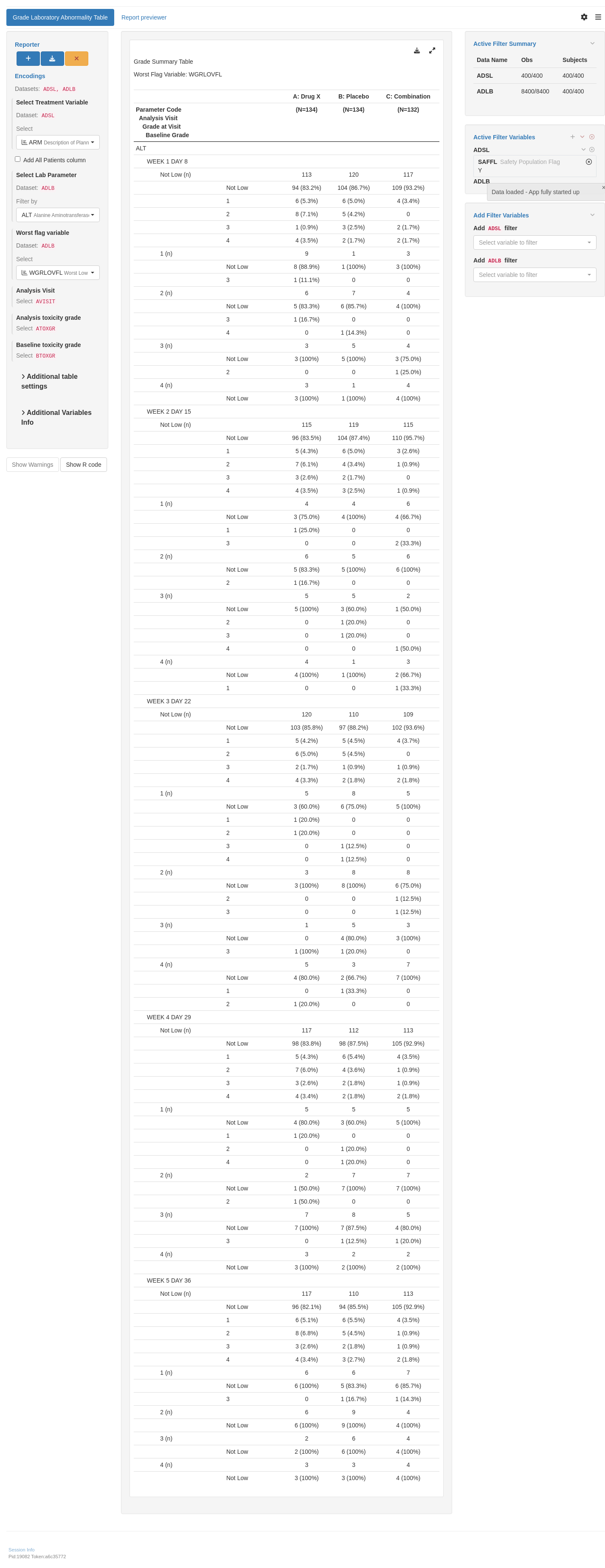
## `teal` App

::: {.panel-tabset .nav-justified}
## {{< fa regular file-lines fa-sm fa-fw >}} Preview

```{r teal, opts.label = c("skip_if_testing", "app")}
library(teal.modules.clinical)

## Data reproducible code
data <- teal_data()
data <- within(data, {
  ADSL <- random.cdisc.data::cadsl
  ADLB <- random.cdisc.data::cadlb
})
datanames <- c("ADSL", "ADLB")
datanames(data) <- datanames
join_keys(data) <- default_cdisc_join_keys[datanames]

## Reusable Configuration For Modules
ADSL <- data[["ADSL"]]
ADLB <- data[["ADLB"]]

## Setup App
app <- init(
  data = data,
  modules = modules(
    tm_t_shift_by_grade(
      label = "Grade Laboratory Abnormality Table",
      dataname = "ADLB",
      arm_var = choices_selected(
        choices = variable_choices(ADSL, subset = c("ARM", "ARMCD")),
        selected = "ARM"
      ),
      paramcd = choices_selected(
        choices = value_choices(ADLB, "PARAMCD", "PARAM"),
        selected = "ALT"
      ),
      worst_flag_var = choices_selected(
        choices = variable_choices(ADLB, subset = c("WGRLOVFL", "WGRLOFL", "WGRHIVFL", "WGRHIFL")),
        selected = c("WGRLOVFL")
      ),
      worst_flag_indicator = choices_selected(
        value_choices(ADLB, "WGRLOVFL"),
        selected = "Y", fixed = TRUE
      ),
      anl_toxgrade_var = choices_selected(
        choices = variable_choices(ADLB, subset = c("ATOXGR")),
        selected = c("ATOXGR"),
        fixed = TRUE
      ),
      base_toxgrade_var = choices_selected(
        choices = variable_choices(ADLB, subset = c("BTOXGR")),
        selected = c("BTOXGR"),
        fixed = TRUE
      ),
      add_total = FALSE
    )
  ),
  filter = teal_slices(teal_slice("ADSL", "SAFFL", selected = "Y"))
)

shinyApp(app$ui, app$server)
```

{{< include ../../_utils/shinylive.qmd >}}
:::

{{< include ../../repro.qmd >}}

Made with ❤️ by the NEST Team

  • Edit this page
  • Report an issue
Cookie Preferences