BWG01

Box Plot

Preview
Try this using WebR

Code

bp_1 <- ggplot(adlb, aes(x = ARMCD, y = AVAL)) +
  stat_summary(geom = "boxplot", fun.data = five_num, fill = fc, color = oc) +
  stat_summary(geom = "point", fun = mean, size = 3, shape = 8) +
  labs(
    title = "Box Plot of Laboratory Test Results",
    subtitle = paste("Visit:", adlb$AVISIT[1]),
    caption = "The whiskers extend to the minimum and maximum values.",
    x = "Treatment Group",
    y = paste0(adlb$PARAMCD[1], " (", adlb$AVALU[1], ")")
  ) +
  theme_bp

plot <- bp_annos(bp_1, oc)
plot

Experimental use!

WebR is a tool allowing you to run R code in the web browser. Modify the code below and click run to see the results. Alternatively, copy the code and click here to open WebR in a new tab.

Preview
Try this using WebR

Code

bp_3 <- ggplot(adlb, aes(x = ARMCD, y = AVAL)) +
  stat_summary(
    geom = "boxplot", fun.data = five_num,
    fun.args = list(probs = c(0.05, 0.25, 0.5, 0.75, 0.95)), fill = fc, color = oc
  ) +
  stat_summary(geom = "point", fun = mean, size = 3, shape = 8) +
  labs(
    title = "Box Plot of Laboratory Test Results",
    subtitle = paste("Visit:", adlb$AVISIT[1]),
    caption = "The whiskers extend to the 5th and 95th percentile. Values outside the whiskers have not been plotted.",
    x = "Treatment Group",
    y = paste0(adlb$PARAMCD[1], " (", adlb$AVALU[1], ")")
  ) +
  theme_bp

plot <- bp_annos(bp_3, oc)
plot

Experimental use!

WebR is a tool allowing you to run R code in the web browser. Modify the code below and click run to see the results. Alternatively, copy the code and click here to open WebR in a new tab.

Preview
Try this using WebR

Code

bp_4 <- ggplot(adlb, aes(x = ARMCD, y = AVAL)) +
  stat_summary(
    geom = "boxplot", fun.data = five_num,
    fun.args = list(probs = c(0.05, 0.25, 0.5, 0.75, 0.95)), fill = fc, color = oc
  ) +
  stat_summary(geom = "point", fun = get_outliers, shape = 1) +
  stat_summary(geom = "point", fun = mean, size = 3, shape = 8) +
  labs(
    title = "Box Plot of Laboratory Test Results",
    subtitle = paste("Visit:", adlb$AVISIT[1]),
    caption = "The whiskers extend to the 5th and 95th percentile.",
    x = "Treatment Group",
    y = paste0(adlb$PARAMCD[1], " (", adlb$AVALU[1], ")")
  ) +
  theme_bp

plot <- bp_annos(bp_4, oc)
plot

Experimental use!

WebR is a tool allowing you to run R code in the web browser. Modify the code below and click run to see the results. Alternatively, copy the code and click here to open WebR in a new tab.

Preview
Try this using WebR

Code

adlb_o <- adlb %>%
  group_by(ARMCD) %>%
  mutate(OUTLIER = AVAL < quantile(AVAL, 0.01) | AVAL > quantile(AVAL, 0.99)) %>%
  filter(OUTLIER == TRUE) %>%
  select(ARMCD, AVAL, USUBJID)
# Next step may be study-specific: shorten USUBJID to make annotation labels
# next 2 lines of code split USUBJID by "-" and take the last syllable as ID
n_split <- max(vapply(strsplit(adlb_o$USUBJID, "-"), length, numeric(1)))
adlb_o$ID <- vapply(strsplit(adlb_o$USUBJID, "-"), `[[`, n_split, FUN.VALUE = "a")

bp_5 <- ggplot(adlb, aes(x = ARMCD, y = AVAL)) +
  stat_summary(
    geom = "boxplot", fun.data = five_num,
    fun.args = list(probs = c(0.01, 0.25, 0.5, 0.75, 0.99)), fill = fc, color = oc
  ) +
  stat_summary(geom = "point", fun = mean, size = 3, shape = 8) +
  geom_point(data = adlb_o, aes(x = ARMCD, y = AVAL), shape = 1) +
  geom_text(data = adlb_o, aes(x = ARMCD, y = AVAL, label = ID), size = 3, hjust = -0.2) +
  labs(
    title = "Box Plot of Laboratory Test Results",
    subtitle = paste("Visit:", adlb$AVISIT[1]),
    caption = "The whiskers extend to the largest and smallest observed value within 1.5*IQR.",
    x = "Treatment Group",
    y = paste0(adlb$PARAMCD[1], " (", adlb$AVALU[1], ")")
  ) +
  theme_bp

plot <- bp_annos(bp_5, oc)
plot

Experimental use!

WebR is a tool allowing you to run R code in the web browser. Modify the code below and click run to see the results. Alternatively, copy the code and click here to open WebR in a new tab.

Preview
Try this using WebR

Code

bp_6 <- ggplot(adlb, aes(x = ARMCD, y = AVAL)) +
  geom_boxplot(fill = fc, color = oc) +
  stat_summary(geom = "point", fun = mean, size = 3, shape = 5) +
  labs(
    title = "Box Plot of Laboratory Test Results",
    subtitle = paste("Visit:", adlb$AVISIT[1]),
    caption = "The whiskers extend to the minimum and maximum values.",
    x = "Treatment Group",
    y = paste0(adlb$PARAMCD[1], " (", adlb$AVALU[1], ")")
  ) +
  theme_bp

plot <- bp_annos(bp_6, oc)
plot

Experimental use!

WebR is a tool allowing you to run R code in the web browser. Modify the code below and click run to see the results. Alternatively, copy the code and click here to open WebR in a new tab.

Preview
Try this using WebR

Code

adsl <- random.cdisc.data::cadsl
adlb <- random.cdisc.data::cadlb

adlb_v <- adlb %>%
  filter(PARAMCD == "ALT" & AVISIT %in% c("WEEK 1 DAY 8", "WEEK 2 DAY 15", "WEEK 3 DAY 22", "WEEK 4 DAY 29"))

bp_7 <- ggplot(adlb_v, aes(x = AVISIT, y = AVAL)) +
  stat_summary(
    geom = "boxplot",
    fun.data = five_num,
    position = position_dodge2(.5),
    aes(fill = ARMCD, color = ARMCD)
  ) +
  stat_summary(
    geom = "point",
    fun = mean,
    aes(group = ARMCD),
    size = 3,
    shape = 8,
    position = position_dodge2(1)
  ) +
  labs(
    title = "Box Plot of Laboratory Test Results",
    caption = "The whiskers extend to the minimum and maximum values.",
    x = "Visit",
    y = paste0(adlb$PARAMCD[1], " (", adlb$AVALU[1], ")")
  ) +
  theme_bp

plot <- bp_annos(bp_7, oc, 2)
plot

Experimental use!

WebR is a tool allowing you to run R code in the web browser. Modify the code below and click run to see the results. Alternatively, copy the code and click here to open WebR in a new tab.

Preview
Try this using WebR

Code

bp_8 <- ggplot(adlb_v, aes(x = ARMCD, y = AVAL)) +
  stat_summary(
    geom = "boxplot",
    fun.data = five_num,
    position = position_dodge2(width = .5),
    aes(fill = AVISIT, color = AVISIT)
  ) +
  stat_summary(
    geom = "point",
    fun = mean,
    aes(group = AVISIT),
    size = 3,
    shape = 8,
    position = position_dodge2(1)
  ) +
  labs(
    title = "Box Plot of Laboratory Test Results",
    caption = "The whiskers extend to the minimum and maximum values.",
    x = "Treatment Group",
    y = paste0(adlb$PARAMCD[1], " (", adlb$AVALU[1], ")")
  ) +
  theme_bp

plot <- bp_annos(bp_8, oc, 2)
plot

Experimental use!

WebR is a tool allowing you to run R code in the web browser. Modify the code below and click run to see the results. Alternatively, copy the code and click here to open WebR in a new tab.

Preview
Try this using WebR

Code

# Make wide dataset with summary statistics
adlb_wide <- adlb %>%
  group_by(ARMCD) %>%
  summarise(
    n = n(),
    mean = round(mean(AVAL), 1),
    median = round(median(AVAL), 1),
    median_ci = paste(round(DescTools::MedianCI(AVAL)[1:2], 1), collapse = " - "),
    q1_q3 = paste(round(quantile(AVAL, c(0.25, 0.75)), 1), collapse = " - "),
    min_max = paste0(round(min(AVAL), 1), "-", max(round(AVAL, 2)))
  )

# Make long dataset
adlb_long <- tidyr::gather(adlb_wide, key = type, value = stat, n:min_max)
adlb_long <- adlb_long %>% mutate(
  type_lbl = case_when(
    type == "n" ~ "n",
    type == "mean" ~ "Mean",
    type == "median" ~ "Median",
    type == "median_ci" ~ "95% CI for Median",
    type == "q1_q3" ~ "25% and 75%-ile",
    type == "min_max" ~ "Min - Max"
  )
)
adlb_long$type_lbl <- factor(adlb_long$type_lbl,
  levels = c("Min - Max", "25% and 75%-ile", "95% CI for Median", "Median", "Mean", "n")
)

bp_9 <- ggplot(adlb, aes(x = ARMCD, y = AVAL)) +
  stat_summary(geom = "boxplot", fun.data = five_num, fill = fc, color = oc) +
  stat_summary(geom = "point", fun = mean, size = 3, shape = 8) +
  labs(
    title = "Box Plot of Laboratory Test Results",
    subtitle = paste("Visit:", adlb$AVISIT[1]),
    x = "Treatment Group",
    y = paste0(adlb$PARAMCD[1], " (", adlb$AVALU[1], ")")
  ) +
  theme_bp

tbl_theme <- theme(
  panel.border = element_blank(),
  panel.grid.major = element_blank(),
  panel.grid.minor = element_blank(),
  axis.ticks = element_blank(),
  axis.title = element_blank(),
  axis.text.y = element_text(face = "plain"),
  axis.text.x = element_blank()
)

tbl_1 <- ggplot(adlb_long, aes(x = ARMCD, y = type_lbl, label = stat), vjust = 10) +
  geom_text(size = 3) +
  scale_y_discrete(labels = levels(adlb_long$type_lbl)) +
  theme_bw() +
  tbl_theme +
  labs(caption = "The whiskers extend to the minimum and maximum values.") +
  theme_bp

plot <- cowplot::plot_grid(bp_annos(bp_9, oc), tbl_1,
  rel_heights = c(4, 2),
  ncol = 1, nrow = 2, align = "v"
)
plot

Experimental use!

WebR is a tool allowing you to run R code in the web browser. Modify the code below and click run to see the results. Alternatively, copy the code and click here to open WebR in a new tab.

Preview
Try this using WebR

Code

tbl_2 <- adlb_long %>%
  filter(type == "n") %>%
  ggplot(aes(x = ARMCD, y = type_lbl, label = stat)) +
  geom_text(size = 3) +
  scale_y_discrete(labels = "n") +
  theme_bw() +
  tbl_theme +
  labs(caption = "The whiskers extend to the minimum and maximum values.") +
  theme_bp

plot <- cowplot::plot_grid(bp_annos(bp_9, oc), tbl_2,
  rel_heights = c(6, 1),
  ncol = 1, nrow = 2, align = "v"
)
plot

Experimental use!

WebR is a tool allowing you to run R code in the web browser. Modify the code below and click run to see the results. Alternatively, copy the code and click here to open WebR in a new tab.

Code

library(dplyr)
library(ggplot2)
library(nestcolor)

adlb <- random.cdisc.data::cadlb
adlb <- adlb %>% filter(PARAMCD == "ALT" & AVISIT == "WEEK 2 DAY 15")

# Definition of boxplot boundaries and whiskers
five_num <- function(x, probs = c(0, 0.25, 0.5, 0.75, 1)) {
  r <- quantile(x, probs)
  names(r) <- c("ymin", "lower", "middle", "upper", "ymax")
  r
}

# get outliers based on quantile
# for outliers based on IQR see coef in geom_boxplot
get_outliers <- function(x, probs = c(0.05, 0.95)) {
  r <- subset(x, x < quantile(x, probs[1]) | quantile(x, probs[2]) < x)
  if (!is.null(x)) {
    x_names <- subset(names(x), x < quantile(x, probs[1]) | quantile(x, probs[2]) < x)
    names(r) <- x_names
  }
  r
}

# create theme used for all plots
theme_bp <- theme(
  plot.title = element_text(hjust = 0),
  plot.subtitle = element_text(hjust = 0),
  plot.caption = element_text(hjust = 0),
  panel.background = element_rect(fill = "white", color = "grey50")
)

# assign fill color and outline color
fc <- "#eaeef5"
oc <- getOption("ggplot2.discrete.fill")[1]

# get plot metadata data to derive coordinates for adding annotations
bp_annos <- function(bp, color, annos = 1) {
  bp_mdat <- ggplot_build(bp)$data[[1]]
  if (annos == 1) {
    bp <- bp +
      geom_segment(data = bp_mdat, aes(
        x = xmin + (xmax - xmin) / 4, xend = xmax - (xmax - xmin) / 4,
        y = ymax, yend = ymax
      ), linewidth = .5, color = color) +
      geom_segment(data = bp_mdat, aes(
        x = xmin + (xmax - xmin) / 4, xend = xmax - (xmax - xmin) / 4,
        y = ymin, yend = ymin
      ), linewidth = .5, color = color)
  } else {
    bp <- bp +
      geom_segment(data = bp_mdat, aes(
        x = xmin + (xmax - xmin) / 4, xend = xmax - (xmax - xmin) / 4,
        y = ymax, yend = ymax
      ), linewidth = .5, color = color) +
      geom_segment(data = bp_mdat, aes(
        x = xmin + (xmax - xmin) / 4, xend = xmax - (xmax - xmin) / 4,
        y = ymin, yend = ymin
      ), linewidth = .5, color = color) +
      geom_segment(data = bp_mdat, aes(
        x = xmin, xend = xmax,
        y = middle, yend = middle
      ), colour = color, linewidth = .5)
  }
  return(bp)
}

Code

library(teal.modules.general)

## Data reproducible code
data <- teal_data()
data <- within(data, {
  library(tern)

  ADSL <- random.cdisc.data::cadsl
  ADLB <- random.cdisc.data::cadlb

  # If PARAMCD and AVISIT are not factors, convert to factors
  # Also fill in missing values with "<Missing>"
  ADLB <- ADLB %>%
    df_explicit_na(
      omit_columns = setdiff(names(ADLB), c("PARAMCD", "AVISIT")),
      char_as_factor = TRUE
    )

  # If statment below fails, pre-process ADLB to be one record per
  # study, subject, param and visit eg. filter with ANLFL = 'Y'
  stopifnot(nrow(ADLB) == nrow(unique(ADLB[, c("STUDYID", "USUBJID", "PARAMCD", "AVISIT")])))
})
datanames <- c("ADSL", "ADLB")
datanames(data) <- datanames
join_keys(data) <- default_cdisc_join_keys[datanames]

## Reusable Configuration For Modules
ADSL <- data[["ADSL"]]
ADLB <- data[["ADLB"]]

## Setup App
app <- init(
  data = data,
  modules = modules(
    tm_g_bivariate(
      x = data_extract_spec(
        dataname = "ADSL",
        select = select_spec(
          label = "Select variable:",
          choices = names(ADSL),
          selected = "ARMCD",
          fixed = FALSE
        )
      ),
      y = data_extract_spec(
        dataname = "ADLB",
        filter = list(
          filter_spec(
            vars = c("PARAMCD"),
            choices = levels(ADLB$PARAMCD),
            selected = levels(ADLB$PARAMCD)[1],
            multiple = FALSE,
            label = "Choose lab parameter"
          ),
          filter_spec(
            vars = c("AVISIT"),
            choices = levels(ADLB$AVISIT),
            selected = levels(ADLB$AVISIT)[1],
            multiple = FALSE,
            label = "Choose visit"
          )
        ),
        select = select_spec(
          label = "Select variable:",
          choices = names(ADLB),
          selected = "AVAL",
          multiple = FALSE,
          fixed = TRUE
        )
      ),
      row_facet = data_extract_spec(
        dataname = "ADLB",
        select = select_spec(
          label = "Select variables:",
          choices = names(ADLB),
          selected = NULL,
          multiple = FALSE,
          fixed = FALSE
        )
      ),
      col_facet = data_extract_spec(
        dataname = "ADLB",
        select = select_spec(
          label = "Select variables:",
          choices = names(ADLB),
          selected = NULL,
          multiple = FALSE,
          fixed = FALSE
        )
      )
    )
  )
)

shinyApp(app$ui, app$server)

Warning: Removed 8000 rows containing non-finite outside the scale range
(`stat_boxplot()`).

Experimental use!

shinylive allow you to modify to run shiny application entirely in the web browser. Modify the code below and click re-run the app to see the results. The performance is slighly worse and some of the features (e.g. downloading) might not work at all.

#| standalone: true
#| viewerHeight: 800
#| editorHeight: 200
#| components: [viewer, editor]
#| layout: vertical

# -- WEBR HELPERS --
options(webr_pkg_repos = c("r-universe" = "https://insightsengineering.r-universe.dev", getOption("webr_pkg_repos")))

# -- APP CODE --
library(teal.modules.general)

## Data reproducible code
data <- teal_data()
data <- within(data, {
  library(tern)

  ADSL <- random.cdisc.data::cadsl
  ADLB <- random.cdisc.data::cadlb

  # If PARAMCD and AVISIT are not factors, convert to factors
  # Also fill in missing values with "<Missing>"
  ADLB <- ADLB %>%
    df_explicit_na(
      omit_columns = setdiff(names(ADLB), c("PARAMCD", "AVISIT")),
      char_as_factor = TRUE
    )

  # If statment below fails, pre-process ADLB to be one record per
  # study, subject, param and visit eg. filter with ANLFL = 'Y'
  stopifnot(nrow(ADLB) == nrow(unique(ADLB[, c("STUDYID", "USUBJID", "PARAMCD", "AVISIT")])))
})
datanames <- c("ADSL", "ADLB")
datanames(data) <- datanames
join_keys(data) <- default_cdisc_join_keys[datanames]

## Reusable Configuration For Modules
ADSL <- data[["ADSL"]]
ADLB <- data[["ADLB"]]

## Setup App
app <- init(
  data = data,
  modules = modules(
    tm_g_bivariate(
      x = data_extract_spec(
        dataname = "ADSL",
        select = select_spec(
          label = "Select variable:",
          choices = names(ADSL),
          selected = "ARMCD",
          fixed = FALSE
        )
      ),
      y = data_extract_spec(
        dataname = "ADLB",
        filter = list(
          filter_spec(
            vars = c("PARAMCD"),
            choices = levels(ADLB$PARAMCD),
            selected = levels(ADLB$PARAMCD)[1],
            multiple = FALSE,
            label = "Choose lab parameter"
          ),
          filter_spec(
            vars = c("AVISIT"),
            choices = levels(ADLB$AVISIT),
            selected = levels(ADLB$AVISIT)[1],
            multiple = FALSE,
            label = "Choose visit"
          )
        ),
        select = select_spec(
          label = "Select variable:",
          choices = names(ADLB),
          selected = "AVAL",
          multiple = FALSE,
          fixed = TRUE
        )
      ),
      row_facet = data_extract_spec(
        dataname = "ADLB",
        select = select_spec(
          label = "Select variables:",
          choices = names(ADLB),
          selected = NULL,
          multiple = FALSE,
          fixed = FALSE
        )
      ),
      col_facet = data_extract_spec(
        dataname = "ADLB",
        select = select_spec(
          label = "Select variables:",
          choices = names(ADLB),
          selected = NULL,
          multiple = FALSE,
          fixed = FALSE
        )
      )
    )
  )
)

shinyApp(app$ui, app$server)

Reproducibility

Timestamp

[1] "2024-11-02 17:55:57 UTC"

Session Info

─ Session info ───────────────────────────────────────────────────────────────
 setting  value
 version  R version 4.4.1 (2024-06-14)
 os       Ubuntu 22.04.5 LTS
 system   x86_64, linux-gnu
 ui       X11
 language (EN)
 collate  en_US.UTF-8
 ctype    en_US.UTF-8
 tz       Etc/UTC
 date     2024-11-02
 pandoc   3.4 @ /usr/bin/ (via rmarkdown)

─ Packages ───────────────────────────────────────────────────────────────────
 package              * version date (UTC) lib source
 backports              1.5.0   2024-05-23 [1] CRAN (R 4.4.1)
 boot                   1.3-31  2024-08-28 [2] CRAN (R 4.4.1)
 brio                   1.1.5   2024-04-24 [1] CRAN (R 4.4.1)
 broom                  1.0.7   2024-09-26 [1] CRAN (R 4.4.1)
 bslib                  0.8.0   2024-07-29 [1] CRAN (R 4.4.1)
 cachem                 1.1.0   2024-05-16 [1] CRAN (R 4.4.1)
 callr                  3.7.6   2024-03-25 [1] CRAN (R 4.4.1)
 cellranger             1.1.0   2016-07-27 [1] CRAN (R 4.4.1)
 checkmate              2.3.2   2024-07-29 [1] CRAN (R 4.4.1)
 chromote               0.3.1   2024-08-30 [1] CRAN (R 4.4.1)
 class                  7.3-22  2023-05-03 [2] CRAN (R 4.4.1)
 cli                    3.6.3   2024-06-21 [1] CRAN (R 4.4.1)
 codetools              0.2-20  2024-03-31 [2] CRAN (R 4.4.1)
 colorspace             2.1-1   2024-07-26 [1] CRAN (R 4.4.1)
 cowplot                1.1.3   2024-01-22 [1] CRAN (R 4.4.1)
 data.table             1.16.2  2024-10-10 [1] CRAN (R 4.4.1)
 DescTools              0.99.57 2024-09-25 [1] CRAN (R 4.4.1)
 digest                 0.6.37  2024-08-19 [1] CRAN (R 4.4.1)
 dplyr                * 1.1.4   2023-11-17 [1] CRAN (R 4.4.1)
 e1071                  1.7-16  2024-09-16 [1] CRAN (R 4.4.1)
 evaluate               1.0.1   2024-10-10 [1] CRAN (R 4.4.1)
 Exact                  3.3     2024-07-21 [1] CRAN (R 4.4.1)
 expm                   1.0-0   2024-08-19 [1] CRAN (R 4.4.1)
 fansi                  1.0.6   2023-12-08 [1] CRAN (R 4.4.1)
 farver                 2.1.2   2024-05-13 [1] CRAN (R 4.4.1)
 fastmap                1.2.0   2024-05-15 [1] CRAN (R 4.4.1)
 fontawesome            0.5.2   2023-08-19 [1] CRAN (R 4.4.1)
 forcats                1.0.0   2023-01-29 [1] CRAN (R 4.4.1)
 formatR                1.14    2023-01-17 [1] CRAN (R 4.4.1)
 formatters           * 0.5.9   2024-09-12 [1] CRAN (R 4.4.1)
 generics               0.1.3   2022-07-05 [1] CRAN (R 4.4.1)
 ggmosaic             * 0.3.3   2021-02-23 [1] CRAN (R 4.4.1)
 ggplot2              * 3.5.1   2024-04-23 [1] CRAN (R 4.4.1)
 ggrepel                0.9.6   2024-09-07 [1] CRAN (R 4.4.1)
 gld                    2.6.6   2022-10-23 [1] CRAN (R 4.4.1)
 glue                   1.8.0   2024-09-30 [1] CRAN (R 4.4.1)
 gtable                 0.3.6   2024-10-25 [1] CRAN (R 4.4.1)
 htmltools              0.5.8.1 2024-04-04 [1] CRAN (R 4.4.1)
 htmlwidgets            1.6.4   2023-12-06 [1] CRAN (R 4.4.1)
 httpuv                 1.6.15  2024-03-26 [1] CRAN (R 4.4.1)
 httr                   1.4.7   2023-08-15 [1] CRAN (R 4.4.1)
 jquerylib              0.1.4   2021-04-26 [1] CRAN (R 4.4.1)
 jsonlite               1.8.9   2024-09-20 [1] CRAN (R 4.4.1)
 knitr                  1.48    2024-07-07 [1] CRAN (R 4.4.1)
 labeling               0.4.3   2023-08-29 [1] CRAN (R 4.4.1)
 later                  1.3.2   2023-12-06 [1] CRAN (R 4.4.1)
 lattice                0.22-6  2024-03-20 [2] CRAN (R 4.4.1)
 lazyeval               0.2.2   2019-03-15 [1] CRAN (R 4.4.1)
 lifecycle              1.0.4   2023-11-07 [1] CRAN (R 4.4.1)
 lmom                   3.2     2024-09-30 [1] CRAN (R 4.4.1)
 logger                 0.4.0   2024-10-22 [1] CRAN (R 4.4.1)
 magrittr             * 2.0.3   2022-03-30 [1] CRAN (R 4.4.1)
 MASS                   7.3-61  2024-06-13 [2] CRAN (R 4.4.1)
 Matrix                 1.7-0   2024-04-26 [1] CRAN (R 4.4.1)
 memoise                2.0.1   2021-11-26 [1] CRAN (R 4.4.1)
 mime                   0.12    2021-09-28 [1] CRAN (R 4.4.1)
 munsell                0.5.1   2024-04-01 [1] CRAN (R 4.4.1)
 mvtnorm                1.3-1   2024-09-03 [1] CRAN (R 4.4.1)
 nestcolor            * 0.1.2   2023-06-09 [1] CRAN (R 4.4.1)
 pillar                 1.9.0   2023-03-22 [1] CRAN (R 4.4.1)
 pkgconfig              2.0.3   2019-09-22 [1] CRAN (R 4.4.1)
 plotly                 4.10.4  2024-01-13 [1] CRAN (R 4.4.1)
 processx               3.8.4   2024-03-16 [1] CRAN (R 4.4.1)
 promises               1.3.0   2024-04-05 [1] CRAN (R 4.4.1)
 proxy                  0.4-27  2022-06-09 [1] CRAN (R 4.4.1)
 ps                     1.8.1   2024-10-28 [1] CRAN (R 4.4.1)
 purrr                  1.0.2   2023-08-10 [1] CRAN (R 4.4.1)
 R6                     2.5.1   2021-08-19 [1] CRAN (R 4.4.1)
 ragg                   1.3.3   2024-09-11 [1] CRAN (R 4.4.1)
 random.cdisc.data      0.3.16  2024-11-02 [1] https://insightsengineering.r-universe.dev (R 4.4.1)
 rbibutils              2.3     2024-10-04 [1] CRAN (R 4.4.1)
 Rcpp                   1.0.13  2024-07-17 [1] CRAN (R 4.4.1)
 Rdpack                 2.6.1   2024-08-06 [1] CRAN (R 4.4.1)
 readxl                 1.4.3   2023-07-06 [1] CRAN (R 4.4.1)
 rlang                  1.1.4   2024-06-04 [1] CRAN (R 4.4.1)
 rmarkdown              2.28    2024-08-17 [1] CRAN (R 4.4.1)
 rootSolve              1.8.2.4 2023-09-21 [1] CRAN (R 4.4.1)
 rstudioapi             0.17.1  2024-10-22 [1] CRAN (R 4.4.1)
 rtables              * 0.6.10  2024-09-20 [1] CRAN (R 4.4.1)
 sass                   0.4.9   2024-03-15 [1] CRAN (R 4.4.1)
 scales                 1.3.0   2023-11-28 [1] CRAN (R 4.4.1)
 sessioninfo            1.2.2   2021-12-06 [1] CRAN (R 4.4.1)
 shiny                * 1.9.1   2024-08-01 [1] CRAN (R 4.4.1)
 shinycssloaders        1.1.0   2024-07-30 [1] CRAN (R 4.4.1)
 shinyjs                2.1.0   2021-12-23 [1] CRAN (R 4.4.1)
 shinyvalidate          0.1.3   2023-10-04 [1] CRAN (R 4.4.1)
 shinyWidgets           0.8.7   2024-09-23 [1] CRAN (R 4.4.1)
 stringi                1.8.4   2024-05-06 [1] CRAN (R 4.4.1)
 stringr                1.5.1   2023-11-14 [1] CRAN (R 4.4.1)
 survival               3.7-0   2024-06-05 [2] CRAN (R 4.4.1)
 systemfonts            1.1.0   2024-05-15 [1] CRAN (R 4.4.1)
 teal                 * 0.15.2  2024-03-07 [1] CRAN (R 4.4.1)
 teal.code            * 0.5.0   2024-01-11 [1] CRAN (R 4.4.1)
 teal.data            * 0.6.0   2024-04-30 [1] CRAN (R 4.4.1)
 teal.logger            0.3.0   2024-11-02 [1] https://insightsengineering.r-universe.dev (R 4.4.1)
 teal.modules.general * 0.3.0   2024-03-05 [1] CRAN (R 4.4.1)
 teal.reporter          0.3.1   2024-03-15 [1] CRAN (R 4.4.1)
 teal.slice           * 0.5.1   2024-04-30 [1] CRAN (R 4.4.1)
 teal.transform       * 0.5.0   2024-02-17 [1] CRAN (R 4.4.1)
 teal.widgets           0.4.2   2023-12-14 [1] CRAN (R 4.4.1)
 tern                 * 0.9.6   2024-09-24 [1] CRAN (R 4.4.1)
 testthat               3.2.1.1 2024-04-14 [1] CRAN (R 4.4.1)
 textshaping            0.4.0   2024-05-24 [1] CRAN (R 4.4.1)
 tibble                 3.2.1   2023-03-20 [1] CRAN (R 4.4.1)
 tidyr                  1.3.1   2024-01-24 [1] CRAN (R 4.4.1)
 tidyselect             1.2.1   2024-03-11 [1] CRAN (R 4.4.1)
 utf8                   1.2.4   2023-10-22 [1] CRAN (R 4.4.1)
 vctrs                  0.6.5   2023-12-01 [1] CRAN (R 4.4.1)
 viridisLite            0.4.2   2023-05-02 [1] CRAN (R 4.4.1)
 webshot                0.5.5   2023-06-26 [1] CRAN (R 4.4.1)
 webshot2               0.1.1   2023-08-11 [1] CRAN (R 4.4.1)
 websocket              1.4.2   2024-07-22 [1] CRAN (R 4.4.1)
 withr                  3.0.2   2024-10-28 [1] CRAN (R 4.4.1)
 xfun                   0.49    2024-10-31 [1] CRAN (R 4.4.1)
 xtable                 1.8-4   2019-04-21 [1] CRAN (R 4.4.1)
 yaml                   2.3.10  2024-07-26 [1] CRAN (R 4.4.1)

 [1] /usr/local/lib/R/site-library
 [2] /usr/local/lib/R/library

──────────────────────────────────────────────────────────────────────────────

`.lock` file

Download the .lock file and use renv::restore() on it to recreate environment used to generate this website.

Download

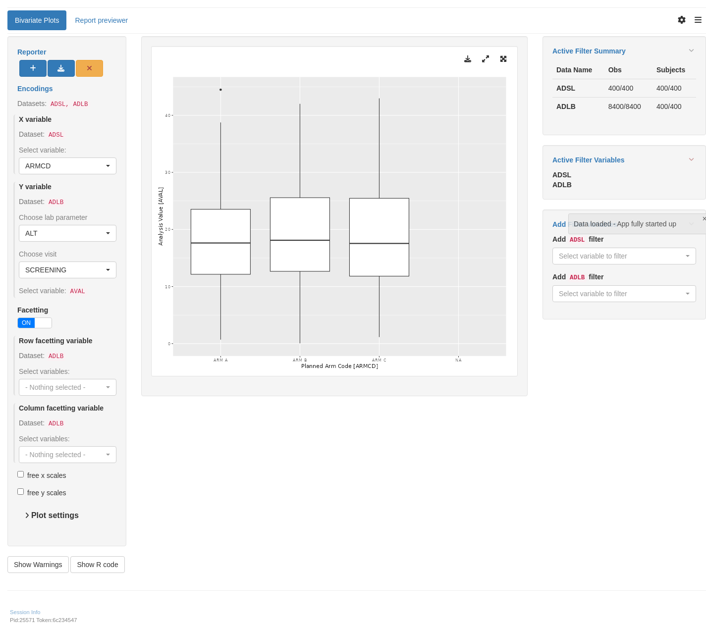
teal App

Reproducibility

Timestamp

Session Info

.lock file

`teal` App

`.lock` file