TLG Catalog - Stable
  • Stable
    • Dev
  1. Tables
  2. Demography
  3. DMT01
  • Introduction

  • Tables
    • ADA
      • ADAT01
      • ADAT02
      • ADAT03
      • ADAT04A
      • ADAT04B
    • Adverse Events
      • AET01
      • AET01_AESI
      • AET02
      • AET02_SMQ
      • AET03
      • AET04
      • AET04_PI
      • AET05
      • AET05_ALL
      • AET06
      • AET06_SMQ
      • AET07
      • AET09
      • AET09_SMQ
      • AET10
    • Concomitant Medications
      • CMT01
      • CMT01A
      • CMT01B
      • CMT02_PT
    • Deaths
      • DTHT01
    • Demography
      • DMT01
    • Disclosures
      • DISCLOSUREST01
      • EUDRAT01
      • EUDRAT02
    • Disposition
      • DST01
      • PDT01
      • PDT02
    • ECG
      • EGT01
      • EGT02
      • EGT03
      • EGT04
      • EGT05_QTCAT
    • Efficacy
      • AOVT01
      • AOVT02
      • AOVT03
      • CFBT01
      • CMHT01
      • COXT01
      • COXT02
      • DORT01
      • LGRT02
      • MMRMT01
      • ONCT05
      • RATET01
      • RBMIT01
      • RSPT01
      • TTET01
    • Exposure
      • EXT01
    • Lab Results
      • LBT01
      • LBT02
      • LBT03
      • LBT04
      • LBT05
      • LBT06
      • LBT07
      • LBT08
      • LBT09
      • LBT10
      • LBT10_BL
      • LBT11
      • LBT11_BL
      • LBT12
      • LBT12_BL
      • LBT13
      • LBT14
      • LBT15
    • Medical History
      • MHT01
    • Pharmacokinetic
      • PKCT01
      • PKPT02
      • PKPT03
      • PKPT04
      • PKPT05
      • PKPT06
      • PKPT07
      • PKPT08
      • PKPT11
    • Risk Management Plan
      • RMPT01
      • RMPT03
      • RMPT04
      • RMPT05
      • RMPT06
    • Safety
      • ENTXX
    • Vital Signs
      • VST01
      • VST02
  • Listings
    • ADA
      • ADAL02
    • Adverse Events
      • AEL01
      • AEL01_NOLLT
      • AEL02
      • AEL02_ED
      • AEL03
      • AEL04
    • Concomitant Medications
      • CML01
      • CML02A_GL
      • CML02B_GL
    • Development Safety Update Report
      • DSUR4
    • Disposition
      • DSL01
      • DSL02
    • ECG
      • EGL01
    • Efficacy
      • ONCL01
    • Exposure
      • EXL01
    • Lab Results
      • LBL01
      • LBL01_RLS
      • LBL02A
      • LBL02A_RLS
      • LBL02B
    • Medical History
      • MHL01
    • Pharmacokinetic
      • ADAL01
      • PKCL01
      • PKCL02
      • PKPL01
      • PKPL02
      • PKPL04
    • Vital Signs
      • VSL01
  • Graphs
    • Efficacy
      • FSTG01
      • FSTG02
      • KMG01
      • MMRMG01
      • MMRMG02
    • Other
      • BRG01
      • BWG01
      • CIG01
      • IPPG01
      • LTG01
      • MNG01
    • Pharmacokinetic
      • PKCG01
      • PKCG02
      • PKCG03
      • PKPG01
      • PKPG02
      • PKPG03
      • PKPG04
      • PKPG06

  • Appendix
    • Reproducibility

  • Index

On this page

  • Output
  • teal App
  • Reproducibility
    • Timestamp
    • Session Info
    • .lock file
  • Edit this page
  • Report an issue
  1. Tables
  2. Demography
  3. DMT01

DMT01

Demographics and Baseline Characteristics


Output

  • Table with an Additional
    Study-Specific Continuous Variable
  • Table with an Additional
    Study-Specific Categorical Variable
  • Table with Subgrouping
    for Some Analyses
  • Table with Additional Vital
    Signs Baseline Values
  • Table with Additional
    Values from ADSUB
  • Data Setup
  • Preview
  • Try this using WebR
Code
vars <- c("AGE", "AGEGR1", "SEX", "ETHNIC", "RACE", "BMRKR1")
var_labels <- c(
  "Age (yr)",
  "Age Group",
  "Sex",
  "Ethnicity",
  "Race",
  "Continous Level Biomarker 1"
)

result <- basic_table(show_colcounts = TRUE) %>%
  split_cols_by(var = "ACTARM") %>%
  add_overall_col("All Patients") %>%
  analyze_vars(
    vars = vars,
    var_labels = var_labels
  ) %>%
  build_table(adsl)

result
                                               A: Drug X    B: Placebo    C: Combination   All Patients
                                                (N=134)       (N=134)        (N=132)         (N=400)   
———————————————————————————————————————————————————————————————————————————————————————————————————————
Age (yr)                                                                                               
  n                                               134           134            132             400     
  Mean (SD)                                   33.8 (6.6)    35.4 (7.9)      35.4 (7.7)      34.9 (7.4) 
  Median                                         33.0          35.0            35.0            34.0    
  Min - Max                                   21.0 - 50.0   21.0 - 62.0    20.0 - 69.0     20.0 - 69.0 
Age Group                                                                                              
  n                                               134           134            132             400     
  18-40                                       113 (84.3%)   103 (76.9%)    106 (80.3%)     322 (80.5%) 
  41-64                                       21 (15.7%)    31 (23.1%)      25 (18.9%)      77 (19.2%) 
  >=65                                             0             0           1 (0.8%)        1 (0.2%)  
Sex                                                                                                    
  n                                               134           134            132             400     
  Female                                       79 (59%)     82 (61.2%)       70 (53%)      231 (57.8%) 
  Male                                         55 (41%)     52 (38.8%)       62 (47%)      169 (42.2%) 
Ethnicity                                                                                              
  n                                               134           134            132             400     
  HISPANIC OR LATINO                          15 (11.2%)    18 (13.4%)      15 (11.4%)       48 (12%)  
  NOT HISPANIC OR LATINO                      104 (77.6%)   103 (76.9%)    101 (76.5%)      308 (77%)  
  NOT REPORTED                                 6 (4.5%)      10 (7.5%)      11 (8.3%)       27 (6.8%)  
  UNKNOWN                                      9 (6.7%)      3 (2.2%)        5 (3.8%)       17 (4.2%)  
Race                                                                                                   
  n                                               134           134            132             400     
  ASIAN                                       68 (50.7%)     67 (50%)       73 (55.3%)      208 (52%)  
  BLACK OR AFRICAN AMERICAN                   31 (23.1%)    28 (20.9%)      32 (24.2%)      91 (22.8%) 
  WHITE                                       27 (20.1%)    26 (19.4%)      21 (15.9%)      74 (18.5%) 
  AMERICAN INDIAN OR ALASKA NATIVE              8 (6%)       11 (8.2%)       6 (4.5%)       25 (6.2%)  
  MULTIPLE                                         0         1 (0.7%)           0            1 (0.2%)  
  NATIVE HAWAIIAN OR OTHER PACIFIC ISLANDER        0         1 (0.7%)           0            1 (0.2%)  
  OTHER                                            0             0              0               0      
  UNKNOWN                                          0             0              0               0      
Continous Level Biomarker 1                                                                            
  n                                               134           134            132             400     
  Mean (SD)                                    6.0 (3.6)     5.7 (3.3)      5.6 (3.5)       5.8 (3.4)  
  Median                                          5.4           4.8            4.6             4.8     
  Min - Max                                   0.4 - 17.7    0.6 - 14.2      0.2 - 21.4      0.2 - 21.4 
Experimental use!

WebR is a tool allowing you to run R code in the web browser. Modify the code below and click run to see the results. Alternatively, copy the code and click here to open WebR in a new tab.

  • Preview
  • Try this using WebR
Code
vars <- c("AGE", "AGEGR1", "SEX", "ETHNIC", "RACE", "BMRKR1_CAT")
var_labels <- c(
  "Age (yr)",
  "Age Group",
  "Sex",
  "Ethnicity",
  "Race",
  "Biomarker 1 Categories"
)

result <- basic_table(show_colcounts = TRUE) %>%
  split_cols_by(var = "ACTARM") %>%
  analyze_vars(
    vars = vars,
    var_labels = var_labels
  ) %>%
  build_table(adsl)

result
                                               A: Drug X    B: Placebo    C: Combination
                                                (N=134)       (N=134)        (N=132)    
————————————————————————————————————————————————————————————————————————————————————————
Age (yr)                                                                                
  n                                               134           134            132      
  Mean (SD)                                   33.8 (6.6)    35.4 (7.9)      35.4 (7.7)  
  Median                                         33.0          35.0            35.0     
  Min - Max                                   21.0 - 50.0   21.0 - 62.0    20.0 - 69.0  
Age Group                                                                               
  n                                               134           134            132      
  18-40                                       113 (84.3%)   103 (76.9%)    106 (80.3%)  
  41-64                                       21 (15.7%)    31 (23.1%)      25 (18.9%)  
  >=65                                             0             0           1 (0.8%)   
Sex                                                                                     
  n                                               134           134            132      
  Female                                       79 (59%)     82 (61.2%)       70 (53%)   
  Male                                         55 (41%)     52 (38.8%)       62 (47%)   
Ethnicity                                                                               
  n                                               134           134            132      
  HISPANIC OR LATINO                          15 (11.2%)    18 (13.4%)      15 (11.4%)  
  NOT HISPANIC OR LATINO                      104 (77.6%)   103 (76.9%)    101 (76.5%)  
  NOT REPORTED                                 6 (4.5%)      10 (7.5%)      11 (8.3%)   
  UNKNOWN                                      9 (6.7%)      3 (2.2%)        5 (3.8%)   
Race                                                                                    
  n                                               134           134            132      
  ASIAN                                       68 (50.7%)     67 (50%)       73 (55.3%)  
  BLACK OR AFRICAN AMERICAN                   31 (23.1%)    28 (20.9%)      32 (24.2%)  
  WHITE                                       27 (20.1%)    26 (19.4%)      21 (15.9%)  
  AMERICAN INDIAN OR ALASKA NATIVE              8 (6%)       11 (8.2%)       6 (4.5%)   
  MULTIPLE                                         0         1 (0.7%)           0       
  NATIVE HAWAIIAN OR OTHER PACIFIC ISLANDER        0         1 (0.7%)           0       
  OTHER                                            0             0              0       
  UNKNOWN                                          0             0              0       
Biomarker 1 Categories                                                                  
  n                                               134           134            132      
  LOW                                         33 (24.6%)    41 (30.6%)      38 (28.8%)  
  MEDIUM                                      84 (62.7%)    76 (56.7%)      80 (60.6%)  
  HIGH                                        17 (12.7%)    17 (12.7%)      14 (10.6%)  
Experimental use!

WebR is a tool allowing you to run R code in the web browser. Modify the code below and click run to see the results. Alternatively, copy the code and click here to open WebR in a new tab.

  • Preview
  • Try this using WebR
Code
split_fun <- drop_split_levels

result <- basic_table(show_colcounts = TRUE) %>%
  split_cols_by(var = "ACTARM") %>%
  analyze_vars(
    vars = c("AGE", "SEX", "RACE"),
    var_labels = c("Age", "Sex", "Race")
  ) %>%
  split_rows_by("STRATA1",
    split_fun = split_fun
  ) %>%
  analyze_vars("BMRKR1") %>%
  build_table(adsl)

result
                                               A: Drug X    B: Placebo    C: Combination
                                                (N=134)       (N=134)        (N=132)    
————————————————————————————————————————————————————————————————————————————————————————
Age                                                                                     
  n                                               134           134            132      
  Mean (SD)                                   33.8 (6.6)    35.4 (7.9)      35.4 (7.7)  
  Median                                         33.0          35.0            35.0     
  Min - Max                                   21.0 - 50.0   21.0 - 62.0    20.0 - 69.0  
Sex                                                                                     
  n                                               134           134            132      
  Female                                       79 (59%)     82 (61.2%)       70 (53%)   
  Male                                         55 (41%)     52 (38.8%)       62 (47%)   
Race                                                                                    
  n                                               134           134            132      
  ASIAN                                       68 (50.7%)     67 (50%)       73 (55.3%)  
  BLACK OR AFRICAN AMERICAN                   31 (23.1%)    28 (20.9%)      32 (24.2%)  
  WHITE                                       27 (20.1%)    26 (19.4%)      21 (15.9%)  
  AMERICAN INDIAN OR ALASKA NATIVE              8 (6%)       11 (8.2%)       6 (4.5%)   
  MULTIPLE                                         0         1 (0.7%)           0       
  NATIVE HAWAIIAN OR OTHER PACIFIC ISLANDER        0         1 (0.7%)           0       
  OTHER                                            0             0              0       
  UNKNOWN                                          0             0              0       
A                                                                                       
  n                                               38            44              40      
  Mean (SD)                                    5.8 (3.8)     5.4 (3.2)      5.1 (3.2)   
  Median                                          5.1           4.5            3.8      
  Min - Max                                   0.4 - 17.7    1.4 - 14.2      1.5 - 14.0  
B                                                                                       
  n                                               47            45              43      
  Mean (SD)                                    6.1 (3.6)     5.8 (3.6)      5.7 (3.4)   
  Median                                          5.2           4.8            5.1      
  Min - Max                                   1.6 - 17.2    0.6 - 13.3      0.2 - 16.5  
C                                                                                       
  n                                               49            45              49      
  Mean (SD)                                    6.0 (3.4)     5.9 (3.2)      6.0 (3.8)   
  Median                                          5.8           5.6            4.5      
  Min - Max                                   0.5 - 15.1    1.5 - 13.9      1.2 - 21.4  
Experimental use!

WebR is a tool allowing you to run R code in the web browser. Modify the code below and click run to see the results. Alternatively, copy the code and click here to open WebR in a new tab.

  • Preview
  • Try this using WebR
Code
result <- basic_table(show_colcounts = TRUE) %>%
  split_cols_by(var = "ACTARM") %>%
  analyze_vars(
    vars = c("AGE", "SEX", "RACE", "DBP", "SBP"),
    var_labels = c(
      "Age (yr)",
      "Sex",
      "Race",
      "Diastolic Blood Pressure",
      "Systolic Blood Pressure"
    )
  ) %>%
  build_table(adsl)

result
                                               A: Drug X      B: Placebo    C: Combination
                                                (N=134)        (N=134)         (N=132)    
——————————————————————————————————————————————————————————————————————————————————————————
Age (yr)                                                                                  
  n                                               134            134             132      
  Mean (SD)                                    33.8 (6.6)     35.4 (7.9)      35.4 (7.7)  
  Median                                          33.0           35.0            35.0     
  Min - Max                                   21.0 - 50.0    21.0 - 62.0     20.0 - 69.0  
Sex                                                                                       
  n                                               134            134             132      
  Female                                        79 (59%)      82 (61.2%)       70 (53%)   
  Male                                          55 (41%)      52 (38.8%)       62 (47%)   
Race                                                                                      
  n                                               134            134             132      
  ASIAN                                        68 (50.7%)      67 (50%)       73 (55.3%)  
  BLACK OR AFRICAN AMERICAN                    31 (23.1%)     28 (20.9%)      32 (24.2%)  
  WHITE                                        27 (20.1%)     26 (19.4%)      21 (15.9%)  
  AMERICAN INDIAN OR ALASKA NATIVE               8 (6%)       11 (8.2%)        6 (4.5%)   
  MULTIPLE                                         0           1 (0.7%)           0       
  NATIVE HAWAIIAN OR OTHER PACIFIC ISLANDER        0           1 (0.7%)           0       
  OTHER                                            0              0               0       
  UNKNOWN                                          0              0               0       
Diastolic Blood Pressure                                                                  
  n                                               134            134             132      
  Mean (SD)                                   96.5 (19.9)    101.1 (19.9)    102.8 (19.5) 
  Median                                          96.0          100.4           102.0     
  Min - Max                                   44.3 - 136.6   29.2 - 143.8    49.4 - 153.5 
Systolic Blood Pressure                                                                   
  n                                               134            134             132      
  Mean (SD)                                   151.7 (31.5)   149.5 (26.5)    144.7 (30.1) 
  Median                                         150.1          153.0           146.5     
  Min - Max                                   69.1 - 231.2   87.2 - 220.9    71.8 - 220.2 
Experimental use!

WebR is a tool allowing you to run R code in the web browser. Modify the code below and click run to see the results. Alternatively, copy the code and click here to open WebR in a new tab.

  • Preview
  • Try this using WebR
Code
result <- basic_table(show_colcounts = TRUE) %>%
  split_cols_by(var = "ACTARM") %>%
  analyze_vars(
    vars = c("AGE", "SEX", "RACE", "BBMISI"),
    var_labels = c(
      "Age (yr)",
      "Sex",
      "Race",
      "Baseline BMI"
    )
  ) %>%
  build_table(adsl)

result
                                               A: Drug X     B: Placebo     C: Combination
                                                (N=134)        (N=134)         (N=132)    
——————————————————————————————————————————————————————————————————————————————————————————
Age (yr)                                                                                  
  n                                               134            134             132      
  Mean (SD)                                   33.8 (6.6)     35.4 (7.9)       35.4 (7.7)  
  Median                                         33.0           35.0             35.0     
  Min - Max                                   21.0 - 50.0    21.0 - 62.0     20.0 - 69.0  
Sex                                                                                       
  n                                               134            134             132      
  Female                                       79 (59%)      82 (61.2%)        70 (53%)   
  Male                                         55 (41%)      52 (38.8%)        62 (47%)   
Race                                                                                      
  n                                               134            134             132      
  ASIAN                                       68 (50.7%)      67 (50%)        73 (55.3%)  
  BLACK OR AFRICAN AMERICAN                   31 (23.1%)     28 (20.9%)       32 (24.2%)  
  WHITE                                       27 (20.1%)     26 (19.4%)       21 (15.9%)  
  AMERICAN INDIAN OR ALASKA NATIVE              8 (6%)        11 (8.2%)        6 (4.5%)   
  MULTIPLE                                         0          1 (0.7%)            0       
  NATIVE HAWAIIAN OR OTHER PACIFIC ISLANDER        0          1 (0.7%)            0       
  OTHER                                            0              0               0       
  UNKNOWN                                          0              0               0       
Baseline BMI                                                                              
  n                                               134            134             132      
  Mean (SD)                                   30.0 (18.3)    32.4 (23.2)     30.1 (18.4)  
  Median                                         27.1           31.1             30.0     
  Min - Max                                   -6.9 - 75.9   -26.6 - 117.9    -44.2 - 87.5 
Experimental use!

WebR is a tool allowing you to run R code in the web browser. Modify the code below and click run to see the results. Alternatively, copy the code and click here to open WebR in a new tab.

Code
library(tern)
library(dplyr)
library(tidyr)

adsl <- random.cdisc.data::cadsl
advs <- random.cdisc.data::cadvs
adsub <- random.cdisc.data::cadsub

# Ensure character variables are converted to factors and empty strings and NAs are explicit missing levels.
adsl <- df_explicit_na(adsl)
advs <- df_explicit_na(advs)
adsub <- df_explicit_na(adsub)

# Change description in variable SEX.
adsl <- adsl %>%
  mutate(
    SEX = factor(case_when(
      SEX == "M" ~ "Male",
      SEX == "F" ~ "Female",
      SEX == "U" ~ "Unknown",
      SEX == "UNDIFFERENTIATED" ~ "Undifferentiated"
    )),
    AGEGR1 = factor(
      case_when(
        between(AGE, 18, 40) ~ "18-40",
        between(AGE, 41, 64) ~ "41-64",
        AGE > 64 ~ ">=65"
      ),
      levels = c("18-40", "41-64", ">=65")
    ),
    BMRKR1_CAT = factor(
      case_when(
        BMRKR1 < 3.5 ~ "LOW",
        BMRKR1 >= 3.5 & BMRKR1 < 10 ~ "MEDIUM",
        BMRKR1 >= 10 ~ "HIGH"
      ),
      levels = c("LOW", "MEDIUM", "HIGH")
    )
  ) %>%
  var_relabel(
    BMRKR1_CAT = "Biomarker 1 Categories"
  )
# The developer needs to do pre-processing to add necessary variables based on ADVS to analysis dataset.
# Obtain SBP, DBP and weight.
get_param_advs <- function(pname, plabel) {
  ds <- advs %>%
    filter(PARAM == plabel & AVISIT == "BASELINE") %>%
    select(USUBJID, AVAL)

  colnames(ds) <- c("USUBJID", pname)

  ds
}
# The developer needs to do pre-processing to add necessary variables based on ADSUB to analysis dataset.
# Obtain baseline BMI (BBMISI).
get_param_adsub <- function(pname, plabel) {
  ds <- adsub %>%
    filter(PARAM == plabel) %>%
    select(USUBJID, AVAL)

  colnames(ds) <- c("USUBJID", pname)

  ds
}
adsl <- adsl %>%
  left_join(get_param_advs("SBP", "Systolic Blood Pressure"), by = "USUBJID") %>%
  left_join(get_param_advs("DBP", "Diastolic Blood Pressure"), by = "USUBJID") %>%
  left_join(get_param_advs("WGT", "Weight"), by = "USUBJID") %>%
  left_join(get_param_adsub("BBMISI", "Baseline BMI"), by = "USUBJID")

teal App

  • Preview
  • Try this using shinylive
Code
library(teal.modules.clinical)

## Data reproducible code
data <- teal_data()
data <- within(data, {
  ADSL <- random.cdisc.data::cadsl

  # Include `EOSDY` and `DCSREAS` variables below because they contain missing data.
  stopifnot(
    any(is.na(ADSL$EOSDY)),
    any(is.na(ADSL$DCSREAS))
  )
})
datanames <- "ADSL"
datanames(data) <- datanames
Warning: `datanames<-()` was deprecated in teal.data 0.7.0.
ℹ invalid to use `datanames()<-` or `names()<-` on an object of class
  `teal_data`. See ?names.teal_data
Code
join_keys(data) <- default_cdisc_join_keys[datanames]

## Setup App
app <- init(
  data = data,
  modules = modules(
    tm_t_summary(
      label = "Demographic Table",
      dataname = "ADSL",
      arm_var = choices_selected(c("ARM", "ARMCD"), "ARM"),
      summarize_vars = choices_selected(
        c("SEX", "RACE", "BMRKR2", "EOSDY", "DCSREAS"),
        c("SEX", "RACE")
      ),
      useNA = "ifany"
    )
  )
)

shinyApp(app$ui, app$server)

Experimental use!

shinylive allow you to modify to run shiny application entirely in the web browser. Modify the code below and click re-run the app to see the results. The performance is slighly worse and some of the features (e.g. downloading) might not work at all.

#| '!! shinylive warning !!': |
#|   shinylive does not work in self-contained HTML documents.
#|   Please set `embed-resources: false` in your metadata.
#| standalone: true
#| viewerHeight: 800
#| editorHeight: 200
#| components: [viewer, editor]
#| layout: vertical

# -- WEBR HELPERS --
options(webr_pkg_repos = c("r-universe" = "https://insightsengineering.r-universe.dev", getOption("webr_pkg_repos")))

# -- APP CODE --
library(teal.modules.clinical)

## Data reproducible code
data <- teal_data()
data <- within(data, {
  ADSL <- random.cdisc.data::cadsl

  # Include `EOSDY` and `DCSREAS` variables below because they contain missing data.
  stopifnot(
    any(is.na(ADSL$EOSDY)),
    any(is.na(ADSL$DCSREAS))
  )
})
datanames <- "ADSL"
datanames(data) <- datanames
join_keys(data) <- default_cdisc_join_keys[datanames]

## Setup App
app <- init(
  data = data,
  modules = modules(
    tm_t_summary(
      label = "Demographic Table",
      dataname = "ADSL",
      arm_var = choices_selected(c("ARM", "ARMCD"), "ARM"),
      summarize_vars = choices_selected(
        c("SEX", "RACE", "BMRKR2", "EOSDY", "DCSREAS"),
        c("SEX", "RACE")
      ),
      useNA = "ifany"
    )
  )
)

shinyApp(app$ui, app$server)

Reproducibility

Timestamp

[1] "2025-07-09 17:50:13 UTC"

Session Info

─ Session info ───────────────────────────────────────────────────────────────
 setting  value
 version  R version 4.5.0 (2025-04-11)
 os       Ubuntu 24.04.2 LTS
 system   x86_64, linux-gnu
 ui       X11
 language (EN)
 collate  en_US.UTF-8
 ctype    en_US.UTF-8
 tz       Etc/UTC
 date     2025-07-09
 pandoc   3.7.0.2 @ /usr/bin/ (via rmarkdown)
 quarto   1.7.32 @ /usr/local/bin/quarto

─ Packages ───────────────────────────────────────────────────────────────────
 package               * version  date (UTC) lib source
 backports               1.5.0    2024-05-23 [1] RSPM
 brio                    1.1.5    2024-04-24 [1] RSPM
 broom                   1.0.8    2025-03-28 [1] RSPM
 bslib                   0.9.0    2025-01-30 [1] RSPM
 cachem                  1.1.0    2024-05-16 [1] RSPM
 callr                   3.7.6    2024-03-25 [1] RSPM
 checkmate               2.3.2    2024-07-29 [1] RSPM
 chromote                0.5.1    2025-04-24 [1] RSPM
 cli                     3.6.5    2025-04-23 [1] RSPM
 coda                    0.19-4.1 2024-01-31 [1] CRAN (R 4.5.0)
 codetools               0.2-20   2024-03-31 [2] CRAN (R 4.5.0)
 curl                    6.4.0    2025-06-22 [1] RSPM
 dichromat               2.0-0.1  2022-05-02 [1] CRAN (R 4.5.0)
 digest                  0.6.37   2024-08-19 [1] RSPM
 dplyr                 * 1.1.4    2023-11-17 [1] RSPM
 emmeans                 1.11.1   2025-05-04 [1] RSPM
 estimability            1.5.1    2024-05-12 [1] RSPM
 evaluate                1.0.4    2025-06-18 [1] RSPM
 farver                  2.1.2    2024-05-13 [1] RSPM
 fastmap                 1.2.0    2024-05-15 [1] RSPM
 fontawesome             0.5.3    2024-11-16 [1] RSPM
 forcats                 1.0.0    2023-01-29 [1] RSPM
 formatR                 1.14     2023-01-17 [1] CRAN (R 4.5.0)
 formatters            * 0.5.11   2025-04-09 [1] RSPM
 geepack                 1.3.12   2024-09-23 [1] RSPM
 generics                0.1.4    2025-05-09 [1] RSPM
 ggplot2                 3.5.2    2025-04-09 [1] RSPM
 glue                    1.8.0    2024-09-30 [1] RSPM
 gtable                  0.3.6    2024-10-25 [1] RSPM
 htmltools               0.5.8.1  2024-04-04 [1] RSPM
 htmlwidgets             1.6.4    2023-12-06 [1] RSPM
 httpuv                  1.6.16   2025-04-16 [1] RSPM
 jquerylib               0.1.4    2021-04-26 [1] RSPM
 jsonlite                2.0.0    2025-03-27 [1] RSPM
 knitr                   1.50     2025-03-16 [1] RSPM
 later                   1.4.2    2025-04-08 [1] RSPM
 lattice                 0.22-7   2025-04-02 [2] CRAN (R 4.5.0)
 lifecycle               1.0.4    2023-11-07 [1] RSPM
 logger                  0.4.0    2024-10-22 [1] RSPM
 magrittr              * 2.0.3    2022-03-30 [1] RSPM
 MASS                    7.3-65   2025-02-28 [2] CRAN (R 4.5.0)
 Matrix                  1.7-3    2025-03-11 [1] CRAN (R 4.5.0)
 memoise                 2.0.1    2021-11-26 [1] RSPM
 mime                    0.13     2025-03-17 [1] RSPM
 multcomp                1.4-28   2025-01-29 [1] RSPM
 mvtnorm                 1.3-3    2025-01-10 [1] RSPM
 nestcolor               0.1.3    2025-01-21 [1] RSPM
 nlme                    3.1-168  2025-03-31 [2] CRAN (R 4.5.0)
 pillar                  1.11.0   2025-07-04 [1] RSPM
 pkgcache                2.2.4    2025-05-26 [1] RSPM
 pkgconfig               2.0.3    2019-09-22 [1] RSPM
 processx                3.8.6    2025-02-21 [1] RSPM
 promises                1.3.3    2025-05-29 [1] RSPM
 ps                      1.9.1    2025-04-12 [1] RSPM
 purrr                   1.0.4    2025-02-05 [1] RSPM
 R6                      2.6.1    2025-02-15 [1] RSPM
 random.cdisc.data       0.3.16   2024-10-10 [1] RSPM
 rbibutils               2.3      2024-10-04 [1] RSPM
 RColorBrewer            1.1-3    2022-04-03 [1] RSPM
 Rcpp                    1.1.0    2025-07-02 [1] RSPM
 Rdpack                  2.6.4    2025-04-09 [1] RSPM
 rlang                   1.1.6    2025-04-11 [1] RSPM
 rmarkdown               2.29     2024-11-04 [1] RSPM
 rtables               * 0.6.13   2025-06-19 [1] RSPM
 sandwich                3.1-1    2024-09-15 [1] RSPM
 sass                    0.4.10   2025-04-11 [1] RSPM
 scales                  1.4.0    2025-04-24 [1] RSPM
 sessioninfo             1.2.3    2025-02-05 [1] any (@1.2.3)
 shiny                 * 1.11.1   2025-07-03 [1] RSPM
 shinycssloaders         1.1.0    2024-07-30 [1] RSPM
 shinyjs                 2.1.0    2021-12-23 [1] RSPM
 shinyvalidate           0.1.3    2023-10-04 [1] RSPM
 shinyWidgets            0.9.0    2025-02-21 [1] RSPM
 stringi                 1.8.7    2025-03-27 [1] RSPM
 stringr                 1.5.1    2023-11-14 [1] RSPM
 survival                3.8-3    2024-12-17 [2] CRAN (R 4.5.0)
 teal                  * 0.16.0   2025-02-23 [1] RSPM
 teal.code             * 0.6.1    2025-02-14 [1] RSPM
 teal.data             * 0.7.0    2025-01-28 [1] RSPM
 teal.logger             0.4.0    2025-07-08 [1] RSPM
 teal.modules.clinical * 0.10.0   2025-02-28 [1] RSPM
 teal.reporter           0.4.0    2025-01-24 [1] RSPM
 teal.slice            * 0.6.0    2025-02-03 [1] RSPM
 teal.transform        * 0.6.0    2025-02-12 [1] RSPM
 teal.widgets            0.4.3    2025-01-31 [1] RSPM
 tern                  * 0.9.9    2025-06-20 [1] RSPM
 tern.gee                0.1.5    2024-08-23 [1] RSPM
 testthat                3.2.3    2025-01-13 [1] RSPM
 TH.data                 1.1-3    2025-01-17 [1] RSPM
 tibble                  3.3.0    2025-06-08 [1] RSPM
 tidyr                 * 1.3.1    2024-01-24 [1] RSPM
 tidyselect              1.2.1    2024-03-11 [1] RSPM
 vctrs                   0.6.5    2023-12-01 [1] RSPM
 webshot                 0.5.5    2023-06-26 [1] CRAN (R 4.5.0)
 webshot2                0.1.2    2025-04-23 [1] RSPM
 websocket               1.4.4    2025-04-10 [1] RSPM
 withr                   3.0.2    2024-10-28 [1] RSPM
 xfun                    0.52     2025-04-02 [1] RSPM
 xtable                  1.8-4    2019-04-21 [1] RSPM
 yaml                    2.3.10   2024-07-26 [1] RSPM
 zoo                     1.8-14   2025-04-10 [1] RSPM

 [1] /usr/local/lib/R/site-library
 [2] /usr/local/lib/R/library
 [3] /github/home/R/x86_64-pc-linux-gnu-library/4.5
 * ── Packages attached to the search path.

──────────────────────────────────────────────────────────────────────────────

.lock file

Download the .lock file and use renv::restore() on it to recreate environment used to generate this website.

Download

DTHT01
DISCLOSUREST01
Source Code
---
title: DMT01
subtitle: Demographics and Baseline Characteristics
---

------------------------------------------------------------------------

{{< include ../../_utils/envir_hook.qmd >}}

```{r setup, echo = FALSE, warning = FALSE, message = FALSE}
library(tern)
library(dplyr)
library(tidyr)

adsl <- random.cdisc.data::cadsl
advs <- random.cdisc.data::cadvs
adsub <- random.cdisc.data::cadsub

# Ensure character variables are converted to factors and empty strings and NAs are explicit missing levels.
adsl <- df_explicit_na(adsl)
advs <- df_explicit_na(advs)
adsub <- df_explicit_na(adsub)

# Change description in variable SEX.
adsl <- adsl %>%
  mutate(
    SEX = factor(case_when(
      SEX == "M" ~ "Male",
      SEX == "F" ~ "Female",
      SEX == "U" ~ "Unknown",
      SEX == "UNDIFFERENTIATED" ~ "Undifferentiated"
    )),
    AGEGR1 = factor(
      case_when(
        between(AGE, 18, 40) ~ "18-40",
        between(AGE, 41, 64) ~ "41-64",
        AGE > 64 ~ ">=65"
      ),
      levels = c("18-40", "41-64", ">=65")
    ),
    BMRKR1_CAT = factor(
      case_when(
        BMRKR1 < 3.5 ~ "LOW",
        BMRKR1 >= 3.5 & BMRKR1 < 10 ~ "MEDIUM",
        BMRKR1 >= 10 ~ "HIGH"
      ),
      levels = c("LOW", "MEDIUM", "HIGH")
    )
  ) %>%
  var_relabel(
    BMRKR1_CAT = "Biomarker 1 Categories"
  )
# The developer needs to do pre-processing to add necessary variables based on ADVS to analysis dataset.
# Obtain SBP, DBP and weight.
get_param_advs <- function(pname, plabel) {
  ds <- advs %>%
    filter(PARAM == plabel & AVISIT == "BASELINE") %>%
    select(USUBJID, AVAL)

  colnames(ds) <- c("USUBJID", pname)

  ds
}
# The developer needs to do pre-processing to add necessary variables based on ADSUB to analysis dataset.
# Obtain baseline BMI (BBMISI).
get_param_adsub <- function(pname, plabel) {
  ds <- adsub %>%
    filter(PARAM == plabel) %>%
    select(USUBJID, AVAL)

  colnames(ds) <- c("USUBJID", pname)

  ds
}
adsl <- adsl %>%
  left_join(get_param_advs("SBP", "Systolic Blood Pressure"), by = "USUBJID") %>%
  left_join(get_param_advs("DBP", "Diastolic Blood Pressure"), by = "USUBJID") %>%
  left_join(get_param_advs("WGT", "Weight"), by = "USUBJID") %>%
  left_join(get_param_adsub("BBMISI", "Baseline BMI"), by = "USUBJID")
```

```{r include = FALSE}
webr_code_labels <- c("setup")
```

{{< include ../../_utils/webr_no_include.qmd >}}

## Output

:::::::: panel-tabset
## Table with an Additional <br/> Study-Specific Continuous Variable

::: {.panel-tabset .nav-justified group="webr"}
## {{< fa regular file-lines sm fw >}} Preview

```{r variant1, test = list(result_v1 = "result")}
vars <- c("AGE", "AGEGR1", "SEX", "ETHNIC", "RACE", "BMRKR1")
var_labels <- c(
  "Age (yr)",
  "Age Group",
  "Sex",
  "Ethnicity",
  "Race",
  "Continous Level Biomarker 1"
)

result <- basic_table(show_colcounts = TRUE) %>%
  split_cols_by(var = "ACTARM") %>%
  add_overall_col("All Patients") %>%
  analyze_vars(
    vars = vars,
    var_labels = var_labels
  ) %>%
  build_table(adsl)

result
```

```{r include = FALSE}
webr_code_labels <- c("variant1")
```

{{< include ../../_utils/webr.qmd >}}
:::

## Table with an Additional <br/> Study-Specific Categorical Variable

::: {.panel-tabset .nav-justified group="webr"}
## {{< fa regular file-lines sm fw >}} Preview

```{r variant2, test = list(result_v2 = "result")}
vars <- c("AGE", "AGEGR1", "SEX", "ETHNIC", "RACE", "BMRKR1_CAT")
var_labels <- c(
  "Age (yr)",
  "Age Group",
  "Sex",
  "Ethnicity",
  "Race",
  "Biomarker 1 Categories"
)

result <- basic_table(show_colcounts = TRUE) %>%
  split_cols_by(var = "ACTARM") %>%
  analyze_vars(
    vars = vars,
    var_labels = var_labels
  ) %>%
  build_table(adsl)

result
```

```{r include = FALSE}
webr_code_labels <- c("variant2")
```

{{< include ../../_utils/webr.qmd >}}
:::

## Table with Subgrouping <br/> for Some Analyses

::: {.panel-tabset .nav-justified group="webr"}
## {{< fa regular file-lines sm fw >}} Preview

```{r variant3, test = list(result_v3 = "result")}
split_fun <- drop_split_levels

result <- basic_table(show_colcounts = TRUE) %>%
  split_cols_by(var = "ACTARM") %>%
  analyze_vars(
    vars = c("AGE", "SEX", "RACE"),
    var_labels = c("Age", "Sex", "Race")
  ) %>%
  split_rows_by("STRATA1",
    split_fun = split_fun
  ) %>%
  analyze_vars("BMRKR1") %>%
  build_table(adsl)

result
```

```{r include = FALSE}
webr_code_labels <- c("variant3")
```

{{< include ../../_utils/webr.qmd >}}
:::

## Table with Additional Vital <br/> Signs Baseline Values

::: {.panel-tabset .nav-justified group="webr"}
## {{< fa regular file-lines sm fw >}} Preview

```{r variant4, test = list(result_v4 = "result")}
result <- basic_table(show_colcounts = TRUE) %>%
  split_cols_by(var = "ACTARM") %>%
  analyze_vars(
    vars = c("AGE", "SEX", "RACE", "DBP", "SBP"),
    var_labels = c(
      "Age (yr)",
      "Sex",
      "Race",
      "Diastolic Blood Pressure",
      "Systolic Blood Pressure"
    )
  ) %>%
  build_table(adsl)

result
```

```{r include = FALSE}
webr_code_labels <- c("variant4")
```

{{< include ../../_utils/webr.qmd >}}
:::

## Table with Additional <br/> Values from ADSUB

::: {.panel-tabset .nav-justified group="webr"}
## {{< fa regular file-lines sm fw >}} Preview

```{r variant5, test = list(result_v5 = "result")}
result <- basic_table(show_colcounts = TRUE) %>%
  split_cols_by(var = "ACTARM") %>%
  analyze_vars(
    vars = c("AGE", "SEX", "RACE", "BBMISI"),
    var_labels = c(
      "Age (yr)",
      "Sex",
      "Race",
      "Baseline BMI"
    )
  ) %>%
  build_table(adsl)

result
```

```{r include = FALSE}
webr_code_labels <- c("variant5")
```

{{< include ../../_utils/webr.qmd >}}
:::

## Data Setup

```{r setup}
#| code-fold: show
```
::::::::

{{< include ../../_utils/save_results.qmd >}}
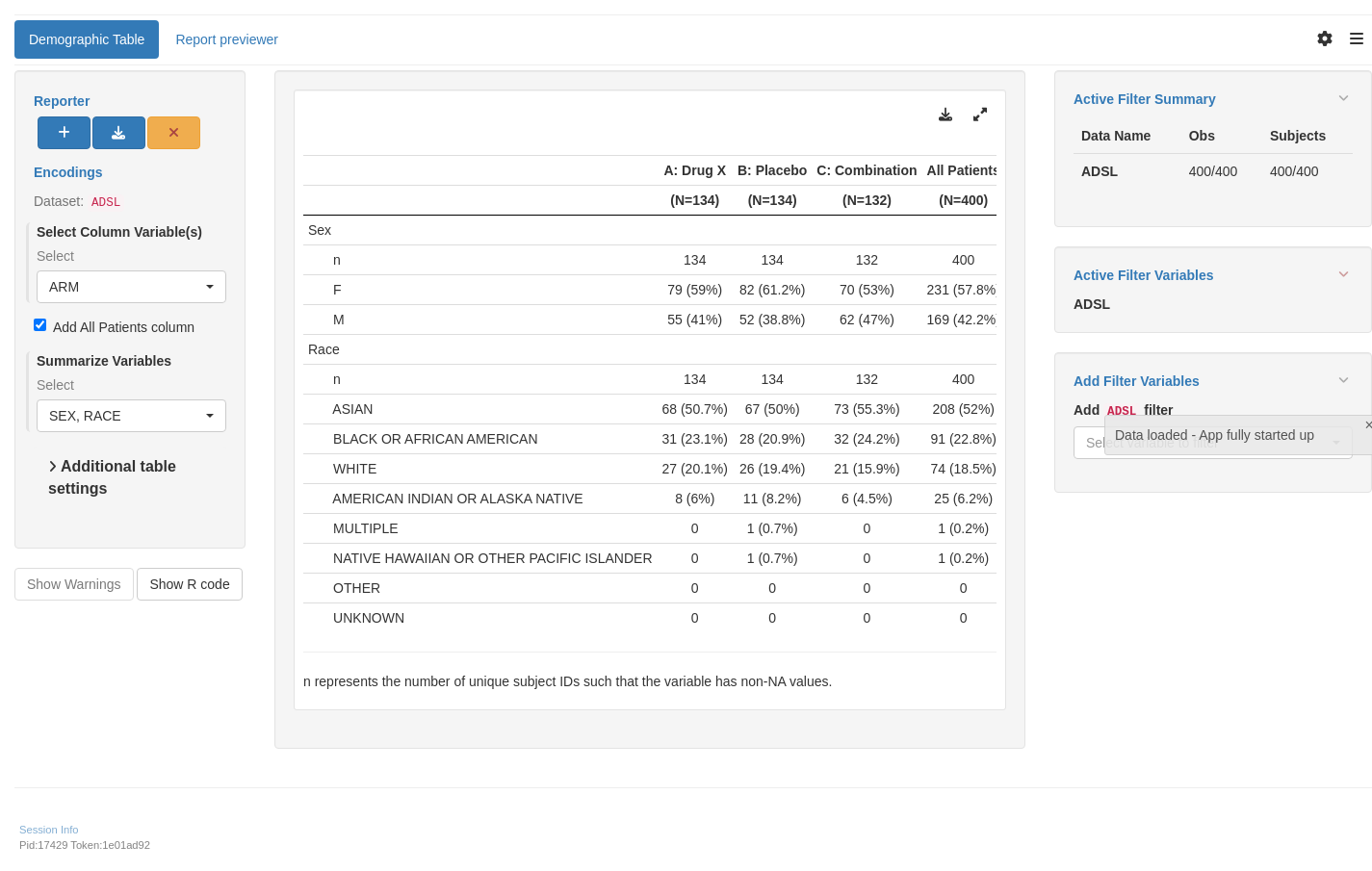
## `teal` App

::: {.panel-tabset .nav-justified}
## {{< fa regular file-lines fa-sm fa-fw >}} Preview

```{r teal, opts.label = c("skip_if_testing", "app")}
library(teal.modules.clinical)

## Data reproducible code
data <- teal_data()
data <- within(data, {
  ADSL <- random.cdisc.data::cadsl

  # Include `EOSDY` and `DCSREAS` variables below because they contain missing data.
  stopifnot(
    any(is.na(ADSL$EOSDY)),
    any(is.na(ADSL$DCSREAS))
  )
})
datanames <- "ADSL"
datanames(data) <- datanames
join_keys(data) <- default_cdisc_join_keys[datanames]

## Setup App
app <- init(
  data = data,
  modules = modules(
    tm_t_summary(
      label = "Demographic Table",
      dataname = "ADSL",
      arm_var = choices_selected(c("ARM", "ARMCD"), "ARM"),
      summarize_vars = choices_selected(
        c("SEX", "RACE", "BMRKR2", "EOSDY", "DCSREAS"),
        c("SEX", "RACE")
      ),
      useNA = "ifany"
    )
  )
)

shinyApp(app$ui, app$server)
```

{{< include ../../_utils/shinylive.qmd >}}
:::

{{< include ../../repro.qmd >}}

Made with ❤️ by the NEST Team

  • Edit this page
  • Report an issue
Cookie Preferences