TLG Catalog - Stable
  • Stable
    • Dev
  1. Tables
  2. Efficacy
  3. COXT01
  • Introduction

  • Tables
    • ADA
      • ADAT01
      • ADAT02
      • ADAT03
      • ADAT04A
      • ADAT04B
    • Adverse Events
      • AET01
      • AET01_AESI
      • AET02
      • AET02_SMQ
      • AET03
      • AET04
      • AET04_PI
      • AET05
      • AET05_ALL
      • AET06
      • AET06_SMQ
      • AET07
      • AET09
      • AET09_SMQ
      • AET10
    • Concomitant Medications
      • CMT01
      • CMT01A
      • CMT01B
      • CMT02_PT
    • Deaths
      • DTHT01
    • Demography
      • DMT01
    • Disclosures
      • DISCLOSUREST01
      • EUDRAT01
      • EUDRAT02
    • Disposition
      • DST01
      • PDT01
      • PDT02
    • ECG
      • EGT01
      • EGT02
      • EGT03
      • EGT04
      • EGT05_QTCAT
    • Efficacy
      • AOVT01
      • AOVT02
      • AOVT03
      • CFBT01
      • CMHT01
      • COXT01
      • COXT02
      • DORT01
      • LGRT02
      • MMRMT01
      • ONCT05
      • RATET01
      • RBMIT01
      • RSPT01
      • TTET01
    • Exposure
      • EXT01
    • Lab Results
      • LBT01
      • LBT02
      • LBT03
      • LBT04
      • LBT05
      • LBT06
      • LBT07
      • LBT08
      • LBT09
      • LBT10
      • LBT10_BL
      • LBT11
      • LBT11_BL
      • LBT12
      • LBT12_BL
      • LBT13
      • LBT14
      • LBT15
    • Medical History
      • MHT01
    • Pharmacokinetic
      • PKCT01
      • PKPT02
      • PKPT03
      • PKPT04
      • PKPT05
      • PKPT06
      • PKPT07
      • PKPT08
      • PKPT11
    • Risk Management Plan
      • RMPT01
      • RMPT03
      • RMPT04
      • RMPT05
      • RMPT06
    • Safety
      • ENTXX
    • Vital Signs
      • VST01
      • VST02
  • Listings
    • ADA
      • ADAL02
    • Adverse Events
      • AEL01
      • AEL01_NOLLT
      • AEL02
      • AEL02_ED
      • AEL03
      • AEL04
    • Concomitant Medications
      • CML01
      • CML02A_GL
      • CML02B_GL
    • Development Safety Update Report
      • DSUR4
    • Disposition
      • DSL01
      • DSL02
    • ECG
      • EGL01
    • Efficacy
      • ONCL01
    • Exposure
      • EXL01
    • Lab Results
      • LBL01
      • LBL01_RLS
      • LBL02A
      • LBL02A_RLS
      • LBL02B
    • Medical History
      • MHL01
    • Pharmacokinetic
      • ADAL01
      • PKCL01
      • PKCL02
      • PKPL01
      • PKPL02
      • PKPL04
    • Vital Signs
      • VSL01
  • Graphs
    • Efficacy
      • FSTG01
      • FSTG02
      • KMG01
      • MMRMG01
      • MMRMG02
    • Other
      • BRG01
      • BWG01
      • CIG01
      • IPPG01
      • LTG01
      • MNG01
    • Pharmacokinetic
      • PKCG01
      • PKCG02
      • PKCG03
      • PKPG01
      • PKPG02
      • PKPG03
      • PKPG04
      • PKPG06

  • Appendix
    • Reproducibility

  • Index

On this page

  • Output
  • teal App
  • Reproducibility
    • Timestamp
    • Session Info
    • .lock file
  • Edit this page
  • Report an issue
  1. Tables
  2. Efficacy
  3. COXT01

COXT01

Cox Regression


Output

Cox models are the most commonly used methods to estimate the magnitude of the effect in survival analyses. It assumes proportional hazards; that is, it assumes that the ratio of the hazards of the two groups (e.g. two arms) is constant over time. This ratio is referred to as the “hazard ratio” and is one of the most commonly reported metrics to describe the effect size in survival analysis.

  • Cox Regression
  • Cox Regression
    with Interaction Term
  • Cox Regression
    Specifying Covariates
  • Cox Regression Setting
    Strata, Ties, Alpha Level
  • Data Setup

The summarize_coxreg function fits, tidies and arranges a Cox regression model in a table layout using the rtables framework. For a Cox regression model, arguments variables, control, and at can be specified (see ?summarize_coxreg for more details and customization options). All variables specified within variables must be present in the data used when building the table.

To see the same model as a data.frame object, these three arguments (as well as the data) can be passed to the fit_coxreg_univar function, and the resulting list tidied using broom::tidy().

  • Preview
  • Try this using WebR
Code
variables <- list(
  time = "AVAL",
  event = "EVENT",
  arm = "ARM",
  covariates = c("AGE", "SEX", "RACE")
)

lyt <- basic_table() %>%
  split_cols_by("col_label") %>%
  summarize_coxreg(variables = variables) %>%
  append_topleft("Effect/Covariate Included in the Model")

result <- build_table(lyt = lyt, df = anl)
result
                                             Treatment Effect Adjusted for Covariate     
Effect/Covariate Included in the Model     n     Hazard Ratio       95% CI       p-value 
—————————————————————————————————————————————————————————————————————————————————————————
Treatment:                                                                               
  A: Drug X vs control (B: Placebo)       247        0.97        (0.66, 1.43)     0.8934 
Covariate:                                                                               
  Age                                     247        0.95        (0.65, 1.40)     0.7948 
  Sex                                     247        0.98        (0.67, 1.43)     0.8970 
  Race                                    247        0.98        (0.67, 1.44)     0.9239 
Experimental use!

WebR is a tool allowing you to run R code in the web browser. Modify the code below and click run to see the results. Alternatively, copy the code and click here to open WebR in a new tab.

The argument control can be used to modify standard outputs; control_coxreg() helps in adopting the right settings (see ?control_coxreg). For instance, control is used to include the interaction terms.

  • Preview
  • Try this using WebR
Code
variables <- list(
  time = "AVAL",
  event = "EVENT",
  arm = "ARM",
  covariates = c("AGE", "RACE")
)

lyt <- basic_table() %>%
  split_cols_by("col_label") %>%
  summarize_coxreg(
    variables = variables,
    control = control_coxreg(interaction = TRUE),
    .stats = c("n", "hr", "ci", "pval", "pval_inter")
  ) %>%
  append_topleft("Effect/Covariate Included in the Model")

result <- build_table(lyt = lyt, df = anl)
result
                                                      Treatment Effect Adjusted for Covariate             
Effect/Covariate Included in the Model    n    Hazard Ratio      95% CI      p-value   Interaction p-value
——————————————————————————————————————————————————————————————————————————————————————————————————————————
Treatment:                                                                                                
  A: Drug X vs control (B: Placebo)      247       0.97       (0.66, 1.43)   0.8934                       
Covariate:                                                                                                
  Age                                    247                                                 0.7878       
    34                                             0.95       (0.65, 1.40)                                
  Race                                   247                                                 0.6850       
    ASIAN                                          1.05       (0.63, 1.75)                                
    BLACK OR AFRICAN AMERICAN                      1.08       (0.51, 2.29)                                
    WHITE                                          0.67       (0.27, 1.71)                                
Experimental use!

WebR is a tool allowing you to run R code in the web browser. Modify the code below and click run to see the results. Alternatively, copy the code and click here to open WebR in a new tab.

The optional argument at allows the user to provide the expected level of estimation for the interaction when the predictor is a quantitative variable. For instance, it might be relevant to choose the age at which the hazard ratio should be estimated. If no input is provided to at, the median value is used in the row name (as in the previous tab).

  • Preview
  • Try this using WebR
Code
variables <- list(
  time = "AVAL",
  event = "EVENT",
  arm = "ARM",
  covariates = c("AGE", "SEX")
)

lyt <- basic_table() %>%
  split_cols_by("col_label") %>%
  summarize_coxreg(
    variables = variables,
    control = control_coxreg(interaction = TRUE),
    at = list(AGE = c(30, 40, 50)),
    .stats = c("n", "hr", "ci", "pval", "pval_inter")
  ) %>%
  append_topleft("Effect/Covariate Included in the Model")

result <- build_table(lyt = lyt, df = anl)
result
                                                      Treatment Effect Adjusted for Covariate             
Effect/Covariate Included in the Model    n    Hazard Ratio      95% CI      p-value   Interaction p-value
——————————————————————————————————————————————————————————————————————————————————————————————————————————
Treatment:                                                                                                
  A: Drug X vs control (B: Placebo)      247       0.97       (0.66, 1.43)   0.8934                       
Covariate:                                                                                                
  Age                                    247                                                 0.7878       
    30                                             0.98       (0.63, 1.51)                                
    40                                             0.91       (0.54, 1.51)                                
    50                                             0.84       (0.32, 2.20)                                
  Sex                                    247                                                 0.1455       
    F                                              0.77       (0.47, 1.27)                                
    M                                              1.38       (0.75, 2.52)                                
Experimental use!

WebR is a tool allowing you to run R code in the web browser. Modify the code below and click run to see the results. Alternatively, copy the code and click here to open WebR in a new tab.

Additional controls can be customized using control_coxreg (see ?control_coxreg) such as the ties calculation method and the confidence level. Stratification variables can be added via the strata element of the variables list.

  • Preview
  • Try this using WebR
Code
variables <- list(
  time = "AVAL",
  event = "EVENT",
  arm = "ARM",
  covariates = c("AGE", "RACE"),
  strata = "SEX"
)

control <- control_coxreg(
  ties = "breslow",
  interaction = TRUE,
  conf_level = 0.90
)

lyt <- basic_table() %>%
  split_cols_by("col_label") %>%
  summarize_coxreg(
    variables = variables,
    control = control,
    at = list(AGE = c(30, 40, 50)),
    .stats = c("n", "hr", "ci", "pval", "pval_inter")
  ) %>%
  append_topleft("Effect/Covariate Included in the Model")

result <- build_table(lyt = lyt, df = anl)
result
                                                      Treatment Effect Adjusted for Covariate             
Effect/Covariate Included in the Model    n    Hazard Ratio      90% CI      p-value   Interaction p-value
——————————————————————————————————————————————————————————————————————————————————————————————————————————
Treatment:                                                                                                
  A: Drug X vs control (B: Placebo)      247       0.98       (0.71, 1.35)   0.9063                       
Covariate:                                                                                                
  Age                                    247                                                 0.7733       
    30                                             0.98       (0.68, 1.42)                                
    40                                             0.91       (0.59, 1.39)                                
    50                                             0.84       (0.38, 1.87)                                
  Race                                   247                                                 0.6501       
    ASIAN                                          1.07       (0.64, 1.77)                                
    BLACK OR AFRICAN AMERICAN                      1.08       (0.51, 2.29)                                
    WHITE                                          0.66       (0.26, 1.67)                                
Experimental use!

WebR is a tool allowing you to run R code in the web browser. Modify the code below and click run to see the results. Alternatively, copy the code and click here to open WebR in a new tab.

Code
library(dplyr)
library(tern)

adsl <- random.cdisc.data::cadsl
adtte <- random.cdisc.data::cadtte

# Ensure character variables are converted to factors and empty strings and NAs are explicit missing levels.
adsl <- df_explicit_na(adsl)
adtte <- df_explicit_na(adtte)

adsl_filtered <- adsl %>% dplyr::filter(
  RACE %in% c("ASIAN", "BLACK OR AFRICAN AMERICAN", "WHITE")
)
adtte_filtered <- dplyr::inner_join(
  x = adsl_filtered[, c("STUDYID", "USUBJID")],
  y = adtte,
  by = c("STUDYID", "USUBJID")
)

anl <- adtte_filtered %>%
  filter(PARAMCD == "OS") %>%
  mutate(EVENT = 1 - CNSR) %>%
  filter(ARM %in% c("B: Placebo", "A: Drug X")) %>%
  mutate(ARM = droplevels(relevel(ARM, "B: Placebo"))) %>%
  mutate(RACE = droplevels(RACE) %>% formatters::with_label("Race"))

# Add variable for column split label
anl <- anl %>% mutate(col_label = "Treatment Effect Adjusted for Covariate")

teal App

  • Preview
  • Try this using shinylive
Code
library(teal.modules.clinical)

arm_ref_comp <- list(
  ACTARMCD = list(
    ref = "ARM B",
    comp = c("ARM A", "ARM C")
  ),
  ARM = list(
    ref = "B: Placebo",
    comp = c("A: Drug X", "C: Combination")
  )
)

## Data reproducible code
data <- teal_data()
data <- within(data, {
  ADSL <- random.cdisc.data::cadsl
  ADTTE <- random.cdisc.data::cadtte

  # Ensure character variables are converted to factors and empty strings and NAs are explicit missing levels.
  ADSL <- df_explicit_na(ADSL)
  ADTTE <- df_explicit_na(ADTTE)
})
datanames <- c("ADSL", "ADTTE")
datanames(data) <- datanames
Warning: `datanames<-()` was deprecated in teal.data 0.7.0.
ℹ invalid to use `datanames()<-` or `names()<-` on an object of class
  `teal_data`. See ?names.teal_data
Code
join_keys(data) <- default_cdisc_join_keys[datanames]

## Reusable Configuration For Modules
ADTTE <- data[["ADTTE"]]

## Setup App
app <- init(
  data = data,
  modules = modules(
    tm_t_coxreg(
      label = "Cox Reg.",
      dataname = "ADTTE",
      arm_var = choices_selected(c("ARM", "ACTARMCD"), "ARM"),
      arm_ref_comp = arm_ref_comp,
      paramcd = choices_selected(
        value_choices(ADTTE, "PARAMCD", "PARAM"), "OS"
      ),
      strata_var = choices_selected(
        c("SEX", "STRATA1", "STRATA2"), NULL
      ),
      cov_var = choices_selected(
        c("AGE", "SEX", "RACE"), "AGE"
      ),
      multivariate = FALSE
    )
  )
)
shinyApp(app$ui, app$server)

Experimental use!

shinylive allow you to modify to run shiny application entirely in the web browser. Modify the code below and click re-run the app to see the results. The performance is slighly worse and some of the features (e.g. downloading) might not work at all.

#| '!! shinylive warning !!': |
#|   shinylive does not work in self-contained HTML documents.
#|   Please set `embed-resources: false` in your metadata.
#| standalone: true
#| viewerHeight: 800
#| editorHeight: 200
#| components: [viewer, editor]
#| layout: vertical

# -- WEBR HELPERS --
options(webr_pkg_repos = c("r-universe" = "https://insightsengineering.r-universe.dev", getOption("webr_pkg_repos")))

# -- APP CODE --
library(teal.modules.clinical)

arm_ref_comp <- list(
  ACTARMCD = list(
    ref = "ARM B",
    comp = c("ARM A", "ARM C")
  ),
  ARM = list(
    ref = "B: Placebo",
    comp = c("A: Drug X", "C: Combination")
  )
)

## Data reproducible code
data <- teal_data()
data <- within(data, {
  ADSL <- random.cdisc.data::cadsl
  ADTTE <- random.cdisc.data::cadtte

  # Ensure character variables are converted to factors and empty strings and NAs are explicit missing levels.
  ADSL <- df_explicit_na(ADSL)
  ADTTE <- df_explicit_na(ADTTE)
})
datanames <- c("ADSL", "ADTTE")
datanames(data) <- datanames
join_keys(data) <- default_cdisc_join_keys[datanames]

## Reusable Configuration For Modules
ADTTE <- data[["ADTTE"]]

## Setup App
app <- init(
  data = data,
  modules = modules(
    tm_t_coxreg(
      label = "Cox Reg.",
      dataname = "ADTTE",
      arm_var = choices_selected(c("ARM", "ACTARMCD"), "ARM"),
      arm_ref_comp = arm_ref_comp,
      paramcd = choices_selected(
        value_choices(ADTTE, "PARAMCD", "PARAM"), "OS"
      ),
      strata_var = choices_selected(
        c("SEX", "STRATA1", "STRATA2"), NULL
      ),
      cov_var = choices_selected(
        c("AGE", "SEX", "RACE"), "AGE"
      ),
      multivariate = FALSE
    )
  )
)
shinyApp(app$ui, app$server)

Reproducibility

Timestamp

[1] "2025-07-05 17:35:18 UTC"

Session Info

─ Session info ───────────────────────────────────────────────────────────────
 setting  value
 version  R version 4.5.0 (2025-04-11)
 os       Ubuntu 24.04.2 LTS
 system   x86_64, linux-gnu
 ui       X11
 language (EN)
 collate  en_US.UTF-8
 ctype    en_US.UTF-8
 tz       Etc/UTC
 date     2025-07-05
 pandoc   3.7.0.2 @ /usr/bin/ (via rmarkdown)
 quarto   1.7.32 @ /usr/local/bin/quarto

─ Packages ───────────────────────────────────────────────────────────────────
 package               * version  date (UTC) lib source
 abind                   1.4-8    2024-09-12 [1] RSPM
 backports               1.5.0    2024-05-23 [1] RSPM
 brio                    1.1.5    2024-04-24 [1] RSPM
 broom                   1.0.8    2025-03-28 [1] RSPM
 bslib                   0.9.0    2025-01-30 [1] RSPM
 cachem                  1.1.0    2024-05-16 [1] RSPM
 callr                   3.7.6    2024-03-25 [1] RSPM
 car                     3.1-3    2024-09-27 [1] RSPM
 carData                 3.0-5    2022-01-06 [1] RSPM
 checkmate               2.3.2    2024-07-29 [1] RSPM
 chromote                0.5.1    2025-04-24 [1] RSPM
 cli                     3.6.5    2025-04-23 [1] RSPM
 coda                    0.19-4.1 2024-01-31 [1] CRAN (R 4.5.0)
 codetools               0.2-20   2024-03-31 [2] CRAN (R 4.5.0)
 curl                    6.4.0    2025-06-22 [1] RSPM
 dichromat               2.0-0.1  2022-05-02 [1] CRAN (R 4.5.0)
 digest                  0.6.37   2024-08-19 [1] RSPM
 dplyr                 * 1.1.4    2023-11-17 [1] RSPM
 emmeans                 1.11.1   2025-05-04 [1] RSPM
 estimability            1.5.1    2024-05-12 [1] RSPM
 evaluate                1.0.4    2025-06-18 [1] RSPM
 farver                  2.1.2    2024-05-13 [1] RSPM
 fastmap                 1.2.0    2024-05-15 [1] RSPM
 fontawesome             0.5.3    2024-11-16 [1] RSPM
 forcats                 1.0.0    2023-01-29 [1] RSPM
 formatR                 1.14     2023-01-17 [1] CRAN (R 4.5.0)
 formatters            * 0.5.11   2025-04-09 [1] RSPM
 Formula                 1.2-5    2023-02-24 [1] RSPM
 geepack                 1.3.12   2024-09-23 [1] RSPM
 generics                0.1.4    2025-05-09 [1] RSPM
 ggplot2                 3.5.2    2025-04-09 [1] RSPM
 glue                    1.8.0    2024-09-30 [1] RSPM
 gtable                  0.3.6    2024-10-25 [1] RSPM
 htmltools               0.5.8.1  2024-04-04 [1] RSPM
 htmlwidgets             1.6.4    2023-12-06 [1] RSPM
 httpuv                  1.6.16   2025-04-16 [1] RSPM
 jquerylib               0.1.4    2021-04-26 [1] RSPM
 jsonlite                2.0.0    2025-03-27 [1] RSPM
 knitr                   1.50     2025-03-16 [1] RSPM
 later                   1.4.2    2025-04-08 [1] RSPM
 lattice                 0.22-7   2025-04-02 [2] CRAN (R 4.5.0)
 lifecycle               1.0.4    2023-11-07 [1] RSPM
 logger                  0.4.0    2024-10-22 [1] RSPM
 magrittr              * 2.0.3    2022-03-30 [1] RSPM
 MASS                    7.3-65   2025-02-28 [2] CRAN (R 4.5.0)
 Matrix                  1.7-3    2025-03-11 [1] CRAN (R 4.5.0)
 memoise                 2.0.1    2021-11-26 [1] RSPM
 mime                    0.13     2025-03-17 [1] RSPM
 multcomp                1.4-28   2025-01-29 [1] RSPM
 mvtnorm                 1.3-3    2025-01-10 [1] RSPM
 nestcolor               0.1.3    2025-01-21 [1] RSPM
 nlme                    3.1-168  2025-03-31 [2] CRAN (R 4.5.0)
 pillar                  1.11.0   2025-07-04 [1] RSPM
 pkgcache                2.2.4    2025-05-26 [1] RSPM
 pkgconfig               2.0.3    2019-09-22 [1] RSPM
 processx                3.8.6    2025-02-21 [1] RSPM
 promises                1.3.3    2025-05-29 [1] RSPM
 ps                      1.9.1    2025-04-12 [1] RSPM
 purrr                   1.0.4    2025-02-05 [1] RSPM
 R6                      2.6.1    2025-02-15 [1] RSPM
 random.cdisc.data       0.3.16   2024-10-10 [1] RSPM
 rbibutils               2.3      2024-10-04 [1] RSPM
 RColorBrewer            1.1-3    2022-04-03 [1] RSPM
 Rcpp                    1.1.0    2025-07-02 [1] RSPM
 Rdpack                  2.6.4    2025-04-09 [1] RSPM
 rlang                   1.1.6    2025-04-11 [1] RSPM
 rmarkdown               2.29     2024-11-04 [1] RSPM
 rtables               * 0.6.13   2025-06-19 [1] RSPM
 sandwich                3.1-1    2024-09-15 [1] RSPM
 sass                    0.4.10   2025-04-11 [1] RSPM
 scales                  1.4.0    2025-04-24 [1] RSPM
 sessioninfo             1.2.3    2025-02-05 [1] any (@1.2.3)
 shiny                 * 1.11.1   2025-07-03 [1] RSPM
 shinycssloaders         1.1.0    2024-07-30 [1] RSPM
 shinyjs                 2.1.0    2021-12-23 [1] RSPM
 shinyvalidate           0.1.3    2023-10-04 [1] RSPM
 shinyWidgets            0.9.0    2025-02-21 [1] RSPM
 stringi                 1.8.7    2025-03-27 [1] RSPM
 stringr                 1.5.1    2023-11-14 [1] RSPM
 survival                3.8-3    2024-12-17 [2] CRAN (R 4.5.0)
 teal                  * 0.16.0   2025-02-23 [1] RSPM
 teal.code             * 0.6.1    2025-02-14 [1] RSPM
 teal.data             * 0.7.0    2025-01-28 [1] RSPM
 teal.logger             0.3.2    2025-02-14 [1] RSPM
 teal.modules.clinical * 0.10.0   2025-02-28 [1] RSPM
 teal.reporter           0.4.0    2025-01-24 [1] RSPM
 teal.slice            * 0.6.0    2025-02-03 [1] RSPM
 teal.transform        * 0.6.0    2025-02-12 [1] RSPM
 teal.widgets            0.4.3    2025-01-31 [1] RSPM
 tern                  * 0.9.9    2025-06-20 [1] RSPM
 tern.gee                0.1.5    2024-08-23 [1] RSPM
 testthat                3.2.3    2025-01-13 [1] RSPM
 TH.data                 1.1-3    2025-01-17 [1] RSPM
 tibble                  3.3.0    2025-06-08 [1] RSPM
 tidyr                   1.3.1    2024-01-24 [1] RSPM
 tidyselect              1.2.1    2024-03-11 [1] RSPM
 vctrs                   0.6.5    2023-12-01 [1] RSPM
 webshot                 0.5.5    2023-06-26 [1] CRAN (R 4.5.0)
 webshot2                0.1.2    2025-04-23 [1] RSPM
 websocket               1.4.4    2025-04-10 [1] RSPM
 withr                   3.0.2    2024-10-28 [1] RSPM
 xfun                    0.52     2025-04-02 [1] RSPM
 xtable                  1.8-4    2019-04-21 [1] RSPM
 yaml                    2.3.10   2024-07-26 [1] RSPM
 zoo                     1.8-14   2025-04-10 [1] RSPM

 [1] /usr/local/lib/R/site-library
 [2] /usr/local/lib/R/library
 [3] /github/home/R/x86_64-pc-linux-gnu-library/4.5
 * ── Packages attached to the search path.

──────────────────────────────────────────────────────────────────────────────

.lock file

Download the .lock file and use renv::restore() on it to recreate environment used to generate this website.

Download

CMHT01
COXT02
Source Code
---
title: COXT01
subtitle: Cox Regression
---

------------------------------------------------------------------------

{{< include ../../_utils/envir_hook.qmd >}}

```{r setup, echo = FALSE, warning = FALSE, message = FALSE}
library(dplyr)
library(tern)

adsl <- random.cdisc.data::cadsl
adtte <- random.cdisc.data::cadtte

# Ensure character variables are converted to factors and empty strings and NAs are explicit missing levels.
adsl <- df_explicit_na(adsl)
adtte <- df_explicit_na(adtte)

adsl_filtered <- adsl %>% dplyr::filter(
  RACE %in% c("ASIAN", "BLACK OR AFRICAN AMERICAN", "WHITE")
)
adtte_filtered <- dplyr::inner_join(
  x = adsl_filtered[, c("STUDYID", "USUBJID")],
  y = adtte,
  by = c("STUDYID", "USUBJID")
)

anl <- adtte_filtered %>%
  filter(PARAMCD == "OS") %>%
  mutate(EVENT = 1 - CNSR) %>%
  filter(ARM %in% c("B: Placebo", "A: Drug X")) %>%
  mutate(ARM = droplevels(relevel(ARM, "B: Placebo"))) %>%
  mutate(RACE = droplevels(RACE) %>% formatters::with_label("Race"))

# Add variable for column split label
anl <- anl %>% mutate(col_label = "Treatment Effect Adjusted for Covariate")
```

```{r include = FALSE}
webr_code_labels <- c("setup")
```

{{< include ../../_utils/webr_no_include.qmd >}}

## Output

Cox models are the most commonly used methods to estimate the magnitude of the effect in survival analyses. It assumes proportional hazards; that is, it assumes that the ratio of the hazards of the two groups (e.g. two arms) is constant over time. This ratio is referred to as the "hazard ratio" and is one of the most commonly reported metrics to describe the effect size in survival analysis.

::::::: panel-tabset
## Cox Regression

The `summarize_coxreg` function fits, tidies and arranges a Cox regression model in a table layout using the `rtables` framework. For a Cox regression model, arguments `variables`, `control`, and `at` can be specified (see `?summarize_coxreg` for more details and customization options). All variables specified within `variables` must be present in the data used when building the table.

To see the same model as a `data.frame` object, these three arguments (as well as the data) can be passed to the `fit_coxreg_univar` function, and the resulting list tidied using `broom::tidy()`.

::: {.panel-tabset .nav-justified group="webr"}
## {{< fa regular file-lines sm fw >}} Preview

```{r variant1, test = list(result_v1 = "result")}
variables <- list(
  time = "AVAL",
  event = "EVENT",
  arm = "ARM",
  covariates = c("AGE", "SEX", "RACE")
)

lyt <- basic_table() %>%
  split_cols_by("col_label") %>%
  summarize_coxreg(variables = variables) %>%
  append_topleft("Effect/Covariate Included in the Model")

result <- build_table(lyt = lyt, df = anl)
result
```

```{r include = FALSE}
webr_code_labels <- c("variant1")
```

{{< include ../../_utils/webr.qmd >}}
:::

## Cox Regression <br/> with Interaction Term

The argument `control` can be used to modify standard outputs; `control_coxreg()` helps in adopting the right settings (see `?control_coxreg`). For instance, `control` is used to include the interaction terms.

::: {.panel-tabset .nav-justified group="webr"}
## {{< fa regular file-lines sm fw >}} Preview

```{r variant2, test = list(result_v2 = "result")}
variables <- list(
  time = "AVAL",
  event = "EVENT",
  arm = "ARM",
  covariates = c("AGE", "RACE")
)

lyt <- basic_table() %>%
  split_cols_by("col_label") %>%
  summarize_coxreg(
    variables = variables,
    control = control_coxreg(interaction = TRUE),
    .stats = c("n", "hr", "ci", "pval", "pval_inter")
  ) %>%
  append_topleft("Effect/Covariate Included in the Model")

result <- build_table(lyt = lyt, df = anl)
result
```

```{r include = FALSE}
webr_code_labels <- c("variant2")
```

{{< include ../../_utils/webr.qmd >}}
:::

## Cox Regression <br/> Specifying Covariates

The optional argument `at` allows the user to provide the expected level of estimation for the interaction when the predictor is a quantitative variable. For instance, it might be relevant to choose the age at which the hazard ratio should be estimated. If no input is provided to `at`, the median value is used in the row name (as in the previous tab).

::: {.panel-tabset .nav-justified group="webr"}
## {{< fa regular file-lines sm fw >}} Preview

```{r variant3, test = list(result_v3 = "result")}
variables <- list(
  time = "AVAL",
  event = "EVENT",
  arm = "ARM",
  covariates = c("AGE", "SEX")
)

lyt <- basic_table() %>%
  split_cols_by("col_label") %>%
  summarize_coxreg(
    variables = variables,
    control = control_coxreg(interaction = TRUE),
    at = list(AGE = c(30, 40, 50)),
    .stats = c("n", "hr", "ci", "pval", "pval_inter")
  ) %>%
  append_topleft("Effect/Covariate Included in the Model")

result <- build_table(lyt = lyt, df = anl)
result
```

```{r include = FALSE}
webr_code_labels <- c("variant3")
```

{{< include ../../_utils/webr.qmd >}}
:::

## Cox Regression Setting <br/> Strata, Ties, Alpha Level

Additional controls can be customized using `control_coxreg` (see `?control_coxreg`) such as the ties calculation method and the confidence level. Stratification variables can be added via the `strata` element of the `variables` list.

::: {.panel-tabset .nav-justified group="webr"}
## {{< fa regular file-lines sm fw >}} Preview

```{r variant4, test = list(result_v4 = "result")}
variables <- list(
  time = "AVAL",
  event = "EVENT",
  arm = "ARM",
  covariates = c("AGE", "RACE"),
  strata = "SEX"
)

control <- control_coxreg(
  ties = "breslow",
  interaction = TRUE,
  conf_level = 0.90
)

lyt <- basic_table() %>%
  split_cols_by("col_label") %>%
  summarize_coxreg(
    variables = variables,
    control = control,
    at = list(AGE = c(30, 40, 50)),
    .stats = c("n", "hr", "ci", "pval", "pval_inter")
  ) %>%
  append_topleft("Effect/Covariate Included in the Model")

result <- build_table(lyt = lyt, df = anl)
result
```

```{r include = FALSE}
webr_code_labels <- c("variant4")
```

{{< include ../../_utils/webr.qmd >}}
:::

## Data Setup

```{r setup}
#| code-fold: show
```
:::::::

{{< include ../../_utils/save_results.qmd >}}
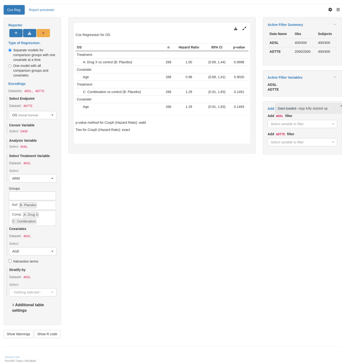
## `teal` App

::: {.panel-tabset .nav-justified}
## {{< fa regular file-lines fa-sm fa-fw >}} Preview

```{r teal, opts.label = c("skip_if_testing", "app")}
library(teal.modules.clinical)

arm_ref_comp <- list(
  ACTARMCD = list(
    ref = "ARM B",
    comp = c("ARM A", "ARM C")
  ),
  ARM = list(
    ref = "B: Placebo",
    comp = c("A: Drug X", "C: Combination")
  )
)

## Data reproducible code
data <- teal_data()
data <- within(data, {
  ADSL <- random.cdisc.data::cadsl
  ADTTE <- random.cdisc.data::cadtte

  # Ensure character variables are converted to factors and empty strings and NAs are explicit missing levels.
  ADSL <- df_explicit_na(ADSL)
  ADTTE <- df_explicit_na(ADTTE)
})
datanames <- c("ADSL", "ADTTE")
datanames(data) <- datanames
join_keys(data) <- default_cdisc_join_keys[datanames]

## Reusable Configuration For Modules
ADTTE <- data[["ADTTE"]]

## Setup App
app <- init(
  data = data,
  modules = modules(
    tm_t_coxreg(
      label = "Cox Reg.",
      dataname = "ADTTE",
      arm_var = choices_selected(c("ARM", "ACTARMCD"), "ARM"),
      arm_ref_comp = arm_ref_comp,
      paramcd = choices_selected(
        value_choices(ADTTE, "PARAMCD", "PARAM"), "OS"
      ),
      strata_var = choices_selected(
        c("SEX", "STRATA1", "STRATA2"), NULL
      ),
      cov_var = choices_selected(
        c("AGE", "SEX", "RACE"), "AGE"
      ),
      multivariate = FALSE
    )
  )
)
shinyApp(app$ui, app$server)
```

{{< include ../../_utils/shinylive.qmd >}}
:::

{{< include ../../repro.qmd >}}

Made with ❤️ by the NEST Team

  • Edit this page
  • Report an issue
Cookie Preferences