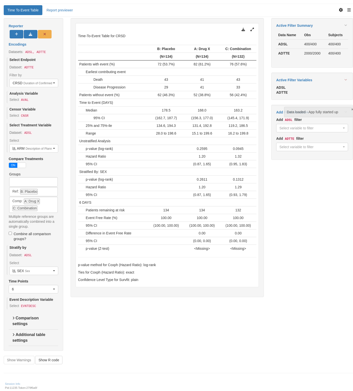
TLG Catalog - Stable
  • Stable
    • Dev
  1. Tables
  2. Efficacy
  3. DORT01
  • Introduction

  • Tables
    • ADA
      • ADAT01
      • ADAT02
      • ADAT03
      • ADAT04A
      • ADAT04B
    • Adverse Events
      • AET01
      • AET01_AESI
      • AET02
      • AET02_SMQ
      • AET03
      • AET04
      • AET04_PI
      • AET05
      • AET05_ALL
      • AET06
      • AET06_SMQ
      • AET07
      • AET09
      • AET09_SMQ
      • AET10
    • Concomitant Medications
      • CMT01
      • CMT01A
      • CMT01B
      • CMT02_PT
    • Deaths
      • DTHT01
    • Demography
      • DMT01
    • Disclosures
      • DISCLOSUREST01
      • EUDRAT01
      • EUDRAT02
    • Disposition
      • DST01
      • PDT01
      • PDT02
    • ECG
      • EGT01
      • EGT02
      • EGT03
      • EGT04
      • EGT05_QTCAT
    • Efficacy
      • AOVT01
      • AOVT02
      • AOVT03
      • CFBT01
      • CMHT01
      • COXT01
      • COXT02
      • DORT01
      • LGRT02
      • MMRMT01
      • ONCT05
      • RATET01
      • RBMIT01
      • RSPT01
      • TTET01
    • Exposure
      • EXT01
    • Lab Results
      • LBT01
      • LBT02
      • LBT03
      • LBT04
      • LBT05
      • LBT06
      • LBT07
      • LBT08
      • LBT09
      • LBT10
      • LBT10_BL
      • LBT11
      • LBT11_BL
      • LBT12
      • LBT12_BL
      • LBT13
      • LBT14
      • LBT15
    • Medical History
      • MHT01
    • Pharmacokinetic
      • PKCT01
      • PKPT02
      • PKPT03
      • PKPT04
      • PKPT05
      • PKPT06
      • PKPT07
      • PKPT08
      • PKPT11
    • Risk Management Plan
      • RMPT01
      • RMPT03
      • RMPT04
      • RMPT05
      • RMPT06
    • Safety
      • ENTXX
    • Vital Signs
      • VST01
      • VST02
  • Listings
    • ADA
      • ADAL02
    • Adverse Events
      • AEL01
      • AEL01_NOLLT
      • AEL02
      • AEL02_ED
      • AEL03
      • AEL04
    • Concomitant Medications
      • CML01
      • CML02A_GL
      • CML02B_GL
    • Development Safety Update Report
      • DSUR4
    • Disposition
      • DSL01
      • DSL02
    • ECG
      • EGL01
    • Efficacy
      • ONCL01
    • Exposure
      • EXL01
    • Lab Results
      • LBL01
      • LBL01_RLS
      • LBL02A
      • LBL02A_RLS
      • LBL02B
    • Medical History
      • MHL01
    • Pharmacokinetic
      • ADAL01
      • PKCL01
      • PKCL02
      • PKPL01
      • PKPL02
      • PKPL04
    • Vital Signs
      • VSL01
  • Graphs
    • Efficacy
      • FSTG01
      • FSTG02
      • KMG01
      • MMRMG01
      • MMRMG02
    • Other
      • BRG01
      • BWG01
      • CIG01
      • IPPG01
      • LTG01
      • MNG01
    • Pharmacokinetic
      • PKCG01
      • PKCG02
      • PKCG03
      • PKPG01
      • PKPG02
      • PKPG03
      • PKPG04
      • PKPG06

  • Appendix
    • Reproducibility

  • Index

On this page

  • Output
  • teal App
  • Reproducibility
    • Timestamp
    • Session Info
    • .lock file
  • Edit this page
  • Report an issue
  1. Tables
  2. Efficacy
  3. DORT01

DORT01

Duration of Response


Output

  • Standard Table
  • Table Selecting
    Sections to Display
  • Table Modifying Analysis Details
    like Conf. Type and Alpha Level
  • Table Modifying Time Point for
    the “XX Months duration” Analysis
  • Data Setup
  • Preview
  • Try this using WebR
Code
lyt <- basic_table(show_colcounts = TRUE) %>%
  split_cols_by(var = "ARM", ref_group = "A: Drug X") %>%
  count_values(
    vars = "USUBJID",
    values = unique(adtte$USUBJID),
    .labels = c(count = "Responders"),
    .stats = "count"
  ) %>%
  analyze_vars(
    vars = "is_event",
    .stats = "count_fraction",
    .labels = c(count_fraction = "Responders with subsequent event (%)"),
    .indent_mods = c(count_fraction = 1L),
    show_labels = "hidden",
  ) %>%
  split_rows_by(
    "EVNT1",
    split_label = "Earliest contributing event",
    split_fun = keep_split_levels("Responders with subsequent event (%)"),
    label_pos = "visible",
    child_labels = "hidden",
    indent_mod = 2L,
  ) %>%
  analyze("EVNTDESC") %>%
  analyze_vars(
    vars = "is_not_event",
    .stats = "count_fraction",
    .labels = c(count_fraction = "Responders without subsequent event (%)"),
    .indent_mods = c(count_fraction = 1L),
    nested = FALSE,
    show_labels = "hidden"
  ) %>%
  surv_time(
    vars = "AVAL",
    var_labels = "Duration of response (Months)",
    is_event = "is_event"
  ) %>%
  surv_timepoint(
    vars = "AVAL",
    var_labels = "Months duration",
    is_event = "is_event",
    time_point = 12
  )

result <- build_table(lyt, df = adtte_f, alt_counts_df = adsl) %>%
  prune_table(prune_func = prune_zeros_only)

result
                                            A: Drug X    B: Placebo   C: Combination
                                             (N=134)      (N=134)        (N=132)    
————————————————————————————————————————————————————————————————————————————————————
Responders                                      68           73             62      
  Responders with subsequent event (%)      46 (67.6%)   39 (53.4%)     32 (51.6%)  
    Earliest contributing event                                                     
      Death                                     26           24             16      
      Disease Progression                       20           15             16      
  Responders without subsequent event (%)   22 (32.4%)   34 (46.6%)     30 (48.4%)  
Duration of response (Months)                                                       
  Median                                       5.3          6.2            5.3      
    95% CI                                  (4.6, 5.8)   (5.4, 6.3)     (4.6, 5.8)  
  25% and 75%-ile                            3.8, 6.3     4.6, 6.4       4.0, 6.1   
  Range                                     0.5 to 6.4   0.9 to 6.5     0.6 to 6.6  
12 Months duration                                                                  
  Patients remaining at risk                    NA           NA             NA      
  Event Free Rate (%)                           NA           NA             NA      
  95% CI                                        NA           NA             NA      
Experimental use!

WebR is a tool allowing you to run R code in the web browser. Modify the code below and click run to see the results. Alternatively, copy the code and click here to open WebR in a new tab.

  • Preview
  • Try this using WebR
Code
lyt <- basic_table(show_colcounts = TRUE) %>%
  split_cols_by(var = "ARM", ref_group = "A: Drug X") %>%
  count_values(
    vars = "USUBJID",
    values = unique(adtte$USUBJID),
    .labels = c(count = "Responders"),
    .stats = "count"
  ) %>%
  analyze_vars(
    vars = "is_event",
    .stats = "count_fraction",
    .labels = c(count_fraction = "Responders with subsequent event (%)"),
    .indent_mods = c(count_fraction = 1L),
    show_labels = "hidden",
  ) %>%
  split_rows_by(
    "EVNT1",
    split_label = "Earliest contributing event",
    split_fun = keep_split_levels("Responders with subsequent event (%)"),
    label_pos = "visible",
    child_labels = "hidden",
    indent_mod = 2L,
  ) %>%
  analyze("EVNTDESC") %>%
  analyze_vars(
    vars = "is_not_event",
    .stats = "count_fraction",
    .labels = c(count_fraction = "Responders without subsequent event (%)"),
    .indent_mods = c(count_fraction = 1L),
    nested = FALSE,
    show_labels = "hidden"
  ) %>%
  surv_time(
    vars = "AVAL",
    var_labels = "Duration of response (Months)",
    is_event = "is_event",
    table_names = "surv_time"
  ) %>%
  coxph_pairwise(
    vars = "AVAL",
    is_event = "is_event",
    var_labels = c("Unstratified Analysis"),
    control = control_coxph(pval_method = "log-rank"),
    table_names = "cox_pair"
  )

result <- build_table(lyt, df = adtte_f, alt_counts_df = adsl) %>%
  prune_table(prune_func = prune_zeros_only)

result
                                            A: Drug X     B: Placebo    C: Combination
                                             (N=134)       (N=134)         (N=132)    
——————————————————————————————————————————————————————————————————————————————————————
Responders                                      68            73              62      
  Responders with subsequent event (%)      46 (67.6%)    39 (53.4%)      32 (51.6%)  
    Earliest contributing event                                                       
      Death                                     26            24              16      
      Disease Progression                       20            15              16      
  Responders without subsequent event (%)   22 (32.4%)    34 (46.6%)      30 (48.4%)  
Duration of response (Months)                                                         
  Median                                       5.3           6.2             5.3      
    95% CI                                  (4.6, 5.8)    (5.4, 6.3)      (4.6, 5.8)  
  25% and 75%-ile                            3.8, 6.3      4.6, 6.4        4.0, 6.1   
  Range                                     0.5 to 6.4    0.9 to 6.5      0.6 to 6.6  
Unstratified Analysis                                                                 
  p-value (log-rank)                                        0.0223          0.6659    
  Hazard Ratio                                               0.60            0.90     
  95% CI                                                 (0.39, 0.93)    (0.57, 1.44) 
Experimental use!

WebR is a tool allowing you to run R code in the web browser. Modify the code below and click run to see the results. Alternatively, copy the code and click here to open WebR in a new tab.

  • Preview
  • Try this using WebR
Code
lyt <- basic_table(show_colcounts = TRUE) %>%
  split_cols_by(var = "ARM", ref_group = "A: Drug X") %>%
  count_values(
    vars = "USUBJID",
    values = unique(adtte$USUBJID),
    .labels = c(count = "Responders"),
    .stats = "count"
  ) %>%
  analyze_vars(
    vars = "is_event",
    .stats = "count_fraction",
    .labels = c(count_fraction = "Responders with subsequent event (%)"),
    .indent_mods = c(count_fraction = 1L),
    show_labels = "hidden",
  ) %>%
  split_rows_by(
    "EVNT1",
    split_label = "Earliest contributing event",
    split_fun = keep_split_levels("Responders with subsequent event (%)"),
    label_pos = "visible",
    child_labels = "hidden",
    indent_mod = 2L,
  ) %>%
  analyze("EVNTDESC") %>%
  analyze_vars(
    vars = "is_not_event",
    .stats = "count_fraction",
    .labels = c(count_fraction = "Responders without subsequent event (%)"),
    .indent_mods = c(count_fraction = 1L),
    nested = FALSE,
    show_labels = "hidden"
  ) %>%
  surv_time(
    vars = "AVAL",
    var_labels = "Duration of response (Months)",
    is_event = "is_event",
    control = control_surv_time(conf_level = 0.90, conf_type = "log-log")
  ) %>%
  surv_timepoint(
    vars = "AVAL",
    var_labels = "Months duration",
    is_event = "is_event",
    time_point = 12,
    control = control_surv_timepoint(conf_level = 0.975)
  )

result <- build_table(lyt, df = adtte_f, alt_counts_df = adsl) %>%
  prune_table(prune_func = prune_zeros_only)

result
                                            A: Drug X    B: Placebo   C: Combination
                                             (N=134)      (N=134)        (N=132)    
————————————————————————————————————————————————————————————————————————————————————
Responders                                      68           73             62      
  Responders with subsequent event (%)      46 (67.6%)   39 (53.4%)     32 (51.6%)  
    Earliest contributing event                                                     
      Death                                     26           24             16      
      Disease Progression                       20           15             16      
  Responders without subsequent event (%)   22 (32.4%)   34 (46.6%)     30 (48.4%)  
Duration of response (Months)                                                       
  Median                                       5.3          6.2            5.3      
    90% CI                                  (4.6, 5.8)   (5.5, 6.3)     (4.6, 5.7)  
  25% and 75%-ile                            3.8, 6.3     4.6, 6.4       4.0, 6.1   
  Range                                     0.5 to 6.4   0.9 to 6.5     0.6 to 6.6  
12 Months duration                                                                  
  Patients remaining at risk                    NA           NA             NA      
  Event Free Rate (%)                           NA           NA             NA      
  97.5% CI                                      NA           NA             NA      
Experimental use!

WebR is a tool allowing you to run R code in the web browser. Modify the code below and click run to see the results. Alternatively, copy the code and click here to open WebR in a new tab.

  • Preview
  • Try this using WebR
Code
lyt <- basic_table(show_colcounts = TRUE) %>%
  split_cols_by(var = "ARM", ref_group = "A: Drug X") %>%
  count_values(
    vars = "USUBJID",
    values = unique(adtte$USUBJID),
    .labels = c(count = "Responders"),
    .stats = "count"
  ) %>%
  analyze_vars(
    vars = "is_event",
    .stats = "count_fraction",
    .labels = c(count_fraction = "Responders with subsequent event (%)"),
    .indent_mods = c(count_fraction = 1L),
    show_labels = "hidden",
  ) %>%
  split_rows_by(
    "EVNT1",
    split_label = "Earliest contributing event",
    split_fun = keep_split_levels("Responders with subsequent event (%)"),
    label_pos = "visible",
    child_labels = "hidden",
    indent_mod = 2L,
  ) %>%
  analyze("EVNTDESC") %>%
  analyze_vars(
    vars = "is_not_event",
    .stats = "count_fraction",
    .labels = c(count_fraction = "Responders without subsequent event (%)"),
    .indent_mods = c(count_fraction = 1L),
    nested = FALSE,
    show_labels = "hidden"
  ) %>%
  surv_time(
    vars = "AVAL",
    var_labels = "Duration of response (Months)",
    is_event = "is_event"
  ) %>%
  surv_timepoint(
    vars = "AVAL",
    var_labels = "Months duration",
    is_event = "is_event",
    time_point = 6
  )

result <- build_table(lyt, df = adtte_f, alt_counts_df = adsl) %>%
  prune_table(prune_func = prune_zeros_only)

result
                                              A: Drug X        B: Placebo     C: Combination
                                               (N=134)          (N=134)          (N=132)    
————————————————————————————————————————————————————————————————————————————————————————————
Responders                                        68               73               62      
  Responders with subsequent event (%)        46 (67.6%)       39 (53.4%)       32 (51.6%)  
    Earliest contributing event                                                             
      Death                                       26               24               16      
      Disease Progression                         20               15               16      
  Responders without subsequent event (%)     22 (32.4%)       34 (46.6%)       30 (48.4%)  
Duration of response (Months)                                                               
  Median                                         5.3              6.2              5.3      
    95% CI                                    (4.6, 5.8)       (5.4, 6.3)       (4.6, 5.8)  
  25% and 75%-ile                              3.8, 6.3         4.6, 6.4         4.0, 6.1   
  Range                                       0.5 to 6.4       0.9 to 6.5       0.6 to 6.6  
6 Months duration                                                                           
  Patients remaining at risk                      10               18               7       
  Event Free Rate (%)                           33.46            50.23            30.56     
  95% CI                                    (20.88, 46.05)   (36.54, 63.92)   (13.56, 47.57)
Experimental use!

WebR is a tool allowing you to run R code in the web browser. Modify the code below and click run to see the results. Alternatively, copy the code and click here to open WebR in a new tab.

Code
library(tern)
library(dplyr)

adsl <- random.cdisc.data::cadsl
adtte <- random.cdisc.data::cadtte

# Ensure character variables are converted to factors and empty strings and NAs are explicit missing levels.
adsl <- df_explicit_na(adsl)
adtte <- df_explicit_na(adtte)

adtte_f <- adtte %>%
  filter(PARAMCD == "CRSD" & BMEASIFL == "Y") %>%
  dplyr::mutate(
    AVAL = day2month(AVAL),
    is_event = CNSR == 0,
    is_not_event = CNSR == 1,
    EVNT1 = factor(
      case_when(
        is_event == TRUE ~ "Responders with subsequent event (%)",
        is_event == FALSE ~ "Responders without subsequent event (%)"
      ),
      levels = c("Responders with subsequent event (%)", "Responders without subsequent event (%)")
    ),
    EVNTDESC = factor(EVNTDESC)
  )

teal App

  • Preview
  • Try this using shinylive
Code
library(teal.modules.clinical)

## Data reproducible code
data <- teal_data()
data <- within(data, {
  ADSL <- random.cdisc.data::cadsl
  ADTTE <- random.cdisc.data::cadtte

  # Ensure character variables are converted to factors and empty strings and NAs are explicit missing levels.
  ADSL <- df_explicit_na(ADSL)
  ADTTE <- df_explicit_na(ADTTE)
})
datanames <- c("ADSL", "ADTTE")
datanames(data) <- datanames
Warning: `datanames<-()` was deprecated in teal.data 0.7.0.
ℹ invalid to use `datanames()<-` or `names()<-` on an object of class
  `teal_data`. See ?names.teal_data
Code
join_keys(data) <- default_cdisc_join_keys[datanames]

## Reusable Configuration For Modules
ADSL <- data[["ADSL"]]
ADTTE <- data[["ADTTE"]]
arm_ref_comp <- list(
  ACTARMCD = list(
    ref = "ARM B",
    comp = c("ARM A", "ARM C")
  ),
  ARM = list(
    ref = "B: Placebo",
    comp = c("A: Drug X", "C: Combination")
  )
)

## Setup App
app <- init(
  data = data,
  modules = modules(
    tm_t_tte(
      label = "Time To Event Table",
      dataname = "ADTTE",
      arm_var = choices_selected(
        variable_choices(ADSL, c("ARM", "ARMCD", "ACTARMCD")),
        "ARM"
      ),
      arm_ref_comp = arm_ref_comp,
      paramcd = choices_selected(
        value_choices(ADTTE, "PARAMCD", "PARAM"),
        "CRSD"
      ),
      strata_var = choices_selected(
        variable_choices(ADSL, c("SEX", "BMRKR2")),
        "SEX"
      ),
      time_points = choices_selected(c(6, 8), 6),
      event_desc_var = choices_selected(
        variable_choices(ADTTE, "EVNTDESC"),
        "EVNTDESC",
        fixed = TRUE
      )
    )
  )
)

shinyApp(app$ui, app$server)

Experimental use!

shinylive allow you to modify to run shiny application entirely in the web browser. Modify the code below and click re-run the app to see the results. The performance is slighly worse and some of the features (e.g. downloading) might not work at all.

#| '!! shinylive warning !!': |
#|   shinylive does not work in self-contained HTML documents.
#|   Please set `embed-resources: false` in your metadata.
#| standalone: true
#| viewerHeight: 800
#| editorHeight: 200
#| components: [viewer, editor]
#| layout: vertical

# -- WEBR HELPERS --
options(webr_pkg_repos = c("r-universe" = "https://insightsengineering.r-universe.dev", getOption("webr_pkg_repos")))

# -- APP CODE --
library(teal.modules.clinical)

## Data reproducible code
data <- teal_data()
data <- within(data, {
  ADSL <- random.cdisc.data::cadsl
  ADTTE <- random.cdisc.data::cadtte

  # Ensure character variables are converted to factors and empty strings and NAs are explicit missing levels.
  ADSL <- df_explicit_na(ADSL)
  ADTTE <- df_explicit_na(ADTTE)
})
datanames <- c("ADSL", "ADTTE")
datanames(data) <- datanames
join_keys(data) <- default_cdisc_join_keys[datanames]

## Reusable Configuration For Modules
ADSL <- data[["ADSL"]]
ADTTE <- data[["ADTTE"]]
arm_ref_comp <- list(
  ACTARMCD = list(
    ref = "ARM B",
    comp = c("ARM A", "ARM C")
  ),
  ARM = list(
    ref = "B: Placebo",
    comp = c("A: Drug X", "C: Combination")
  )
)

## Setup App
app <- init(
  data = data,
  modules = modules(
    tm_t_tte(
      label = "Time To Event Table",
      dataname = "ADTTE",
      arm_var = choices_selected(
        variable_choices(ADSL, c("ARM", "ARMCD", "ACTARMCD")),
        "ARM"
      ),
      arm_ref_comp = arm_ref_comp,
      paramcd = choices_selected(
        value_choices(ADTTE, "PARAMCD", "PARAM"),
        "CRSD"
      ),
      strata_var = choices_selected(
        variable_choices(ADSL, c("SEX", "BMRKR2")),
        "SEX"
      ),
      time_points = choices_selected(c(6, 8), 6),
      event_desc_var = choices_selected(
        variable_choices(ADTTE, "EVNTDESC"),
        "EVNTDESC",
        fixed = TRUE
      )
    )
  )
)

shinyApp(app$ui, app$server)

Reproducibility

Timestamp

[1] "2025-07-05 17:37:08 UTC"

Session Info

─ Session info ───────────────────────────────────────────────────────────────
 setting  value
 version  R version 4.5.0 (2025-04-11)
 os       Ubuntu 24.04.2 LTS
 system   x86_64, linux-gnu
 ui       X11
 language (EN)
 collate  en_US.UTF-8
 ctype    en_US.UTF-8
 tz       Etc/UTC
 date     2025-07-05
 pandoc   3.7.0.2 @ /usr/bin/ (via rmarkdown)
 quarto   1.7.32 @ /usr/local/bin/quarto

─ Packages ───────────────────────────────────────────────────────────────────
 package               * version  date (UTC) lib source
 backports               1.5.0    2024-05-23 [1] RSPM
 brio                    1.1.5    2024-04-24 [1] RSPM
 broom                   1.0.8    2025-03-28 [1] RSPM
 bslib                   0.9.0    2025-01-30 [1] RSPM
 cachem                  1.1.0    2024-05-16 [1] RSPM
 callr                   3.7.6    2024-03-25 [1] RSPM
 checkmate               2.3.2    2024-07-29 [1] RSPM
 chromote                0.5.1    2025-04-24 [1] RSPM
 cli                     3.6.5    2025-04-23 [1] RSPM
 coda                    0.19-4.1 2024-01-31 [1] CRAN (R 4.5.0)
 codetools               0.2-20   2024-03-31 [2] CRAN (R 4.5.0)
 curl                    6.4.0    2025-06-22 [1] RSPM
 dichromat               2.0-0.1  2022-05-02 [1] CRAN (R 4.5.0)
 digest                  0.6.37   2024-08-19 [1] RSPM
 dplyr                 * 1.1.4    2023-11-17 [1] RSPM
 emmeans                 1.11.1   2025-05-04 [1] RSPM
 estimability            1.5.1    2024-05-12 [1] RSPM
 evaluate                1.0.4    2025-06-18 [1] RSPM
 farver                  2.1.2    2024-05-13 [1] RSPM
 fastmap                 1.2.0    2024-05-15 [1] RSPM
 fontawesome             0.5.3    2024-11-16 [1] RSPM
 forcats                 1.0.0    2023-01-29 [1] RSPM
 formatR                 1.14     2023-01-17 [1] CRAN (R 4.5.0)
 formatters            * 0.5.11   2025-04-09 [1] RSPM
 geepack                 1.3.12   2024-09-23 [1] RSPM
 generics                0.1.4    2025-05-09 [1] RSPM
 ggplot2                 3.5.2    2025-04-09 [1] RSPM
 glue                    1.8.0    2024-09-30 [1] RSPM
 gtable                  0.3.6    2024-10-25 [1] RSPM
 htmltools               0.5.8.1  2024-04-04 [1] RSPM
 htmlwidgets             1.6.4    2023-12-06 [1] RSPM
 httpuv                  1.6.16   2025-04-16 [1] RSPM
 jquerylib               0.1.4    2021-04-26 [1] RSPM
 jsonlite                2.0.0    2025-03-27 [1] RSPM
 knitr                   1.50     2025-03-16 [1] RSPM
 later                   1.4.2    2025-04-08 [1] RSPM
 lattice                 0.22-7   2025-04-02 [2] CRAN (R 4.5.0)
 lifecycle               1.0.4    2023-11-07 [1] RSPM
 logger                  0.4.0    2024-10-22 [1] RSPM
 magrittr              * 2.0.3    2022-03-30 [1] RSPM
 MASS                    7.3-65   2025-02-28 [2] CRAN (R 4.5.0)
 Matrix                  1.7-3    2025-03-11 [1] CRAN (R 4.5.0)
 memoise                 2.0.1    2021-11-26 [1] RSPM
 mime                    0.13     2025-03-17 [1] RSPM
 multcomp                1.4-28   2025-01-29 [1] RSPM
 mvtnorm                 1.3-3    2025-01-10 [1] RSPM
 nestcolor               0.1.3    2025-01-21 [1] RSPM
 nlme                    3.1-168  2025-03-31 [2] CRAN (R 4.5.0)
 pillar                  1.11.0   2025-07-04 [1] RSPM
 pkgcache                2.2.4    2025-05-26 [1] RSPM
 pkgconfig               2.0.3    2019-09-22 [1] RSPM
 processx                3.8.6    2025-02-21 [1] RSPM
 promises                1.3.3    2025-05-29 [1] RSPM
 ps                      1.9.1    2025-04-12 [1] RSPM
 purrr                   1.0.4    2025-02-05 [1] RSPM
 R6                      2.6.1    2025-02-15 [1] RSPM
 random.cdisc.data       0.3.16   2024-10-10 [1] RSPM
 rbibutils               2.3      2024-10-04 [1] RSPM
 RColorBrewer            1.1-3    2022-04-03 [1] RSPM
 Rcpp                    1.1.0    2025-07-02 [1] RSPM
 Rdpack                  2.6.4    2025-04-09 [1] RSPM
 rlang                   1.1.6    2025-04-11 [1] RSPM
 rmarkdown               2.29     2024-11-04 [1] RSPM
 rtables               * 0.6.13   2025-06-19 [1] RSPM
 sandwich                3.1-1    2024-09-15 [1] RSPM
 sass                    0.4.10   2025-04-11 [1] RSPM
 scales                  1.4.0    2025-04-24 [1] RSPM
 sessioninfo             1.2.3    2025-02-05 [1] any (@1.2.3)
 shiny                 * 1.11.1   2025-07-03 [1] RSPM
 shinycssloaders         1.1.0    2024-07-30 [1] RSPM
 shinyjs                 2.1.0    2021-12-23 [1] RSPM
 shinyvalidate           0.1.3    2023-10-04 [1] RSPM
 shinyWidgets            0.9.0    2025-02-21 [1] RSPM
 stringi                 1.8.7    2025-03-27 [1] RSPM
 stringr                 1.5.1    2023-11-14 [1] RSPM
 survival                3.8-3    2024-12-17 [2] CRAN (R 4.5.0)
 teal                  * 0.16.0   2025-02-23 [1] RSPM
 teal.code             * 0.6.1    2025-02-14 [1] RSPM
 teal.data             * 0.7.0    2025-01-28 [1] RSPM
 teal.logger             0.3.2    2025-02-14 [1] RSPM
 teal.modules.clinical * 0.10.0   2025-02-28 [1] RSPM
 teal.reporter           0.4.0    2025-01-24 [1] RSPM
 teal.slice            * 0.6.0    2025-02-03 [1] RSPM
 teal.transform        * 0.6.0    2025-02-12 [1] RSPM
 teal.widgets            0.4.3    2025-01-31 [1] RSPM
 tern                  * 0.9.9    2025-06-20 [1] RSPM
 tern.gee                0.1.5    2024-08-23 [1] RSPM
 testthat                3.2.3    2025-01-13 [1] RSPM
 TH.data                 1.1-3    2025-01-17 [1] RSPM
 tibble                  3.3.0    2025-06-08 [1] RSPM
 tidyr                   1.3.1    2024-01-24 [1] RSPM
 tidyselect              1.2.1    2024-03-11 [1] RSPM
 vctrs                   0.6.5    2023-12-01 [1] RSPM
 webshot                 0.5.5    2023-06-26 [1] CRAN (R 4.5.0)
 webshot2                0.1.2    2025-04-23 [1] RSPM
 websocket               1.4.4    2025-04-10 [1] RSPM
 withr                   3.0.2    2024-10-28 [1] RSPM
 xfun                    0.52     2025-04-02 [1] RSPM
 xtable                  1.8-4    2019-04-21 [1] RSPM
 yaml                    2.3.10   2024-07-26 [1] RSPM
 zoo                     1.8-14   2025-04-10 [1] RSPM

 [1] /usr/local/lib/R/site-library
 [2] /usr/local/lib/R/library
 [3] /github/home/R/x86_64-pc-linux-gnu-library/4.5
 * ── Packages attached to the search path.

──────────────────────────────────────────────────────────────────────────────

.lock file

Download the .lock file and use renv::restore() on it to recreate environment used to generate this website.

Download

COXT02
LGRT02
Source Code
---
title: DORT01
subtitle: Duration of Response
---

------------------------------------------------------------------------

{{< include ../../_utils/envir_hook.qmd >}}

```{r setup, echo = FALSE, warning = FALSE, message = FALSE}
library(tern)
library(dplyr)

adsl <- random.cdisc.data::cadsl
adtte <- random.cdisc.data::cadtte

# Ensure character variables are converted to factors and empty strings and NAs are explicit missing levels.
adsl <- df_explicit_na(adsl)
adtte <- df_explicit_na(adtte)

adtte_f <- adtte %>%
  filter(PARAMCD == "CRSD" & BMEASIFL == "Y") %>%
  dplyr::mutate(
    AVAL = day2month(AVAL),
    is_event = CNSR == 0,
    is_not_event = CNSR == 1,
    EVNT1 = factor(
      case_when(
        is_event == TRUE ~ "Responders with subsequent event (%)",
        is_event == FALSE ~ "Responders without subsequent event (%)"
      ),
      levels = c("Responders with subsequent event (%)", "Responders without subsequent event (%)")
    ),
    EVNTDESC = factor(EVNTDESC)
  )
```

```{r include = FALSE}
webr_code_labels <- c("setup")
```

{{< include ../../_utils/webr_no_include.qmd >}}

## Output

::::::: panel-tabset
## Standard Table

::: {.panel-tabset .nav-justified group="webr"}
## {{< fa regular file-lines sm fw >}} Preview

```{r variant1, test = list(result_v1 = "result")}
lyt <- basic_table(show_colcounts = TRUE) %>%
  split_cols_by(var = "ARM", ref_group = "A: Drug X") %>%
  count_values(
    vars = "USUBJID",
    values = unique(adtte$USUBJID),
    .labels = c(count = "Responders"),
    .stats = "count"
  ) %>%
  analyze_vars(
    vars = "is_event",
    .stats = "count_fraction",
    .labels = c(count_fraction = "Responders with subsequent event (%)"),
    .indent_mods = c(count_fraction = 1L),
    show_labels = "hidden",
  ) %>%
  split_rows_by(
    "EVNT1",
    split_label = "Earliest contributing event",
    split_fun = keep_split_levels("Responders with subsequent event (%)"),
    label_pos = "visible",
    child_labels = "hidden",
    indent_mod = 2L,
  ) %>%
  analyze("EVNTDESC") %>%
  analyze_vars(
    vars = "is_not_event",
    .stats = "count_fraction",
    .labels = c(count_fraction = "Responders without subsequent event (%)"),
    .indent_mods = c(count_fraction = 1L),
    nested = FALSE,
    show_labels = "hidden"
  ) %>%
  surv_time(
    vars = "AVAL",
    var_labels = "Duration of response (Months)",
    is_event = "is_event"
  ) %>%
  surv_timepoint(
    vars = "AVAL",
    var_labels = "Months duration",
    is_event = "is_event",
    time_point = 12
  )

result <- build_table(lyt, df = adtte_f, alt_counts_df = adsl) %>%
  prune_table(prune_func = prune_zeros_only)

result
```

```{r include = FALSE}
webr_code_labels <- c("variant1")
```

{{< include ../../_utils/webr.qmd >}}
:::

## Table Selecting <br/> Sections to Display

::: {.panel-tabset .nav-justified group="webr"}
## {{< fa regular file-lines sm fw >}} Preview

```{r variant2, test = list(result_v2 = "result")}
lyt <- basic_table(show_colcounts = TRUE) %>%
  split_cols_by(var = "ARM", ref_group = "A: Drug X") %>%
  count_values(
    vars = "USUBJID",
    values = unique(adtte$USUBJID),
    .labels = c(count = "Responders"),
    .stats = "count"
  ) %>%
  analyze_vars(
    vars = "is_event",
    .stats = "count_fraction",
    .labels = c(count_fraction = "Responders with subsequent event (%)"),
    .indent_mods = c(count_fraction = 1L),
    show_labels = "hidden",
  ) %>%
  split_rows_by(
    "EVNT1",
    split_label = "Earliest contributing event",
    split_fun = keep_split_levels("Responders with subsequent event (%)"),
    label_pos = "visible",
    child_labels = "hidden",
    indent_mod = 2L,
  ) %>%
  analyze("EVNTDESC") %>%
  analyze_vars(
    vars = "is_not_event",
    .stats = "count_fraction",
    .labels = c(count_fraction = "Responders without subsequent event (%)"),
    .indent_mods = c(count_fraction = 1L),
    nested = FALSE,
    show_labels = "hidden"
  ) %>%
  surv_time(
    vars = "AVAL",
    var_labels = "Duration of response (Months)",
    is_event = "is_event",
    table_names = "surv_time"
  ) %>%
  coxph_pairwise(
    vars = "AVAL",
    is_event = "is_event",
    var_labels = c("Unstratified Analysis"),
    control = control_coxph(pval_method = "log-rank"),
    table_names = "cox_pair"
  )

result <- build_table(lyt, df = adtte_f, alt_counts_df = adsl) %>%
  prune_table(prune_func = prune_zeros_only)

result
```

```{r include = FALSE}
webr_code_labels <- c("variant2")
```

{{< include ../../_utils/webr.qmd >}}
:::

## Table Modifying Analysis Details <br/> like Conf. Type and Alpha Level

::: {.panel-tabset .nav-justified group="webr"}
## {{< fa regular file-lines sm fw >}} Preview

```{r variant3, test = list(result_v3 = "result")}
lyt <- basic_table(show_colcounts = TRUE) %>%
  split_cols_by(var = "ARM", ref_group = "A: Drug X") %>%
  count_values(
    vars = "USUBJID",
    values = unique(adtte$USUBJID),
    .labels = c(count = "Responders"),
    .stats = "count"
  ) %>%
  analyze_vars(
    vars = "is_event",
    .stats = "count_fraction",
    .labels = c(count_fraction = "Responders with subsequent event (%)"),
    .indent_mods = c(count_fraction = 1L),
    show_labels = "hidden",
  ) %>%
  split_rows_by(
    "EVNT1",
    split_label = "Earliest contributing event",
    split_fun = keep_split_levels("Responders with subsequent event (%)"),
    label_pos = "visible",
    child_labels = "hidden",
    indent_mod = 2L,
  ) %>%
  analyze("EVNTDESC") %>%
  analyze_vars(
    vars = "is_not_event",
    .stats = "count_fraction",
    .labels = c(count_fraction = "Responders without subsequent event (%)"),
    .indent_mods = c(count_fraction = 1L),
    nested = FALSE,
    show_labels = "hidden"
  ) %>%
  surv_time(
    vars = "AVAL",
    var_labels = "Duration of response (Months)",
    is_event = "is_event",
    control = control_surv_time(conf_level = 0.90, conf_type = "log-log")
  ) %>%
  surv_timepoint(
    vars = "AVAL",
    var_labels = "Months duration",
    is_event = "is_event",
    time_point = 12,
    control = control_surv_timepoint(conf_level = 0.975)
  )

result <- build_table(lyt, df = adtte_f, alt_counts_df = adsl) %>%
  prune_table(prune_func = prune_zeros_only)

result
```

```{r include = FALSE}
webr_code_labels <- c("variant3")
```

{{< include ../../_utils/webr.qmd >}}
:::

## Table Modifying Time Point for <br/> the "XX Months duration" Analysis

::: {.panel-tabset .nav-justified group="webr"}
## {{< fa regular file-lines sm fw >}} Preview

```{r variant4, test = list(result_v4 = "result")}
lyt <- basic_table(show_colcounts = TRUE) %>%
  split_cols_by(var = "ARM", ref_group = "A: Drug X") %>%
  count_values(
    vars = "USUBJID",
    values = unique(adtte$USUBJID),
    .labels = c(count = "Responders"),
    .stats = "count"
  ) %>%
  analyze_vars(
    vars = "is_event",
    .stats = "count_fraction",
    .labels = c(count_fraction = "Responders with subsequent event (%)"),
    .indent_mods = c(count_fraction = 1L),
    show_labels = "hidden",
  ) %>%
  split_rows_by(
    "EVNT1",
    split_label = "Earliest contributing event",
    split_fun = keep_split_levels("Responders with subsequent event (%)"),
    label_pos = "visible",
    child_labels = "hidden",
    indent_mod = 2L,
  ) %>%
  analyze("EVNTDESC") %>%
  analyze_vars(
    vars = "is_not_event",
    .stats = "count_fraction",
    .labels = c(count_fraction = "Responders without subsequent event (%)"),
    .indent_mods = c(count_fraction = 1L),
    nested = FALSE,
    show_labels = "hidden"
  ) %>%
  surv_time(
    vars = "AVAL",
    var_labels = "Duration of response (Months)",
    is_event = "is_event"
  ) %>%
  surv_timepoint(
    vars = "AVAL",
    var_labels = "Months duration",
    is_event = "is_event",
    time_point = 6
  )

result <- build_table(lyt, df = adtte_f, alt_counts_df = adsl) %>%
  prune_table(prune_func = prune_zeros_only)

result
```

```{r include = FALSE}
webr_code_labels <- c("variant4")
```

{{< include ../../_utils/webr.qmd >}}
:::

## Data Setup

```{r setup}
#| code-fold: show
```
:::::::

{{< include ../../_utils/save_results.qmd >}}

## `teal` App

::: {.panel-tabset .nav-justified}
## {{< fa regular file-lines fa-sm fa-fw >}} Preview

```{r teal, opts.label = c("skip_if_testing", "app")}
library(teal.modules.clinical)

## Data reproducible code
data <- teal_data()
data <- within(data, {
  ADSL <- random.cdisc.data::cadsl
  ADTTE <- random.cdisc.data::cadtte

  # Ensure character variables are converted to factors and empty strings and NAs are explicit missing levels.
  ADSL <- df_explicit_na(ADSL)
  ADTTE <- df_explicit_na(ADTTE)
})
datanames <- c("ADSL", "ADTTE")
datanames(data) <- datanames
join_keys(data) <- default_cdisc_join_keys[datanames]

## Reusable Configuration For Modules
ADSL <- data[["ADSL"]]
ADTTE <- data[["ADTTE"]]
arm_ref_comp <- list(
  ACTARMCD = list(
    ref = "ARM B",
    comp = c("ARM A", "ARM C")
  ),
  ARM = list(
    ref = "B: Placebo",
    comp = c("A: Drug X", "C: Combination")
  )
)

## Setup App
app <- init(
  data = data,
  modules = modules(
    tm_t_tte(
      label = "Time To Event Table",
      dataname = "ADTTE",
      arm_var = choices_selected(
        variable_choices(ADSL, c("ARM", "ARMCD", "ACTARMCD")),
        "ARM"
      ),
      arm_ref_comp = arm_ref_comp,
      paramcd = choices_selected(
        value_choices(ADTTE, "PARAMCD", "PARAM"),
        "CRSD"
      ),
      strata_var = choices_selected(
        variable_choices(ADSL, c("SEX", "BMRKR2")),
        "SEX"
      ),
      time_points = choices_selected(c(6, 8), 6),
      event_desc_var = choices_selected(
        variable_choices(ADTTE, "EVNTDESC"),
        "EVNTDESC",
        fixed = TRUE
      )
    )
  )
)

shinyApp(app$ui, app$server)
```

{{< include ../../_utils/shinylive.qmd >}}
:::

{{< include ../../repro.qmd >}}

Made with ❤️ by the NEST Team

  • Edit this page
  • Report an issue
Cookie Preferences