TLG Catalog - Stable
  • Stable
    • Dev
  1. Tables
  2. Efficacy
  3. LGRT02
  • Introduction

  • Tables
    • ADA
      • ADAT01
      • ADAT02
      • ADAT03
      • ADAT04A
      • ADAT04B
    • Adverse Events
      • AET01
      • AET01_AESI
      • AET02
      • AET02_SMQ
      • AET03
      • AET04
      • AET04_PI
      • AET05
      • AET05_ALL
      • AET06
      • AET06_SMQ
      • AET07
      • AET09
      • AET09_SMQ
      • AET10
    • Concomitant Medications
      • CMT01
      • CMT01A
      • CMT01B
      • CMT02_PT
    • Deaths
      • DTHT01
    • Demography
      • DMT01
    • Disclosures
      • DISCLOSUREST01
      • EUDRAT01
      • EUDRAT02
    • Disposition
      • DST01
      • PDT01
      • PDT02
    • ECG
      • EGT01
      • EGT02
      • EGT03
      • EGT04
      • EGT05_QTCAT
    • Efficacy
      • AOVT01
      • AOVT02
      • AOVT03
      • CFBT01
      • CMHT01
      • COXT01
      • COXT02
      • DORT01
      • LGRT02
      • MMRMT01
      • ONCT05
      • RATET01
      • RBMIT01
      • RSPT01
      • TTET01
    • Exposure
      • EXT01
    • Lab Results
      • LBT01
      • LBT02
      • LBT03
      • LBT04
      • LBT05
      • LBT06
      • LBT07
      • LBT08
      • LBT09
      • LBT10
      • LBT10_BL
      • LBT11
      • LBT11_BL
      • LBT12
      • LBT12_BL
      • LBT13
      • LBT14
      • LBT15
    • Medical History
      • MHT01
    • Pharmacokinetic
      • PKCT01
      • PKPT02
      • PKPT03
      • PKPT04
      • PKPT05
      • PKPT06
      • PKPT07
      • PKPT08
      • PKPT11
    • Risk Management Plan
      • RMPT01
      • RMPT03
      • RMPT04
      • RMPT05
      • RMPT06
    • Safety
      • ENTXX
    • Vital Signs
      • VST01
      • VST02
  • Listings
    • ADA
      • ADAL02
    • Adverse Events
      • AEL01
      • AEL01_NOLLT
      • AEL02
      • AEL02_ED
      • AEL03
      • AEL04
    • Concomitant Medications
      • CML01
      • CML02A_GL
      • CML02B_GL
    • Development Safety Update Report
      • DSUR4
    • Disposition
      • DSL01
      • DSL02
    • ECG
      • EGL01
    • Efficacy
      • ONCL01
    • Exposure
      • EXL01
    • Lab Results
      • LBL01
      • LBL01_RLS
      • LBL02A
      • LBL02A_RLS
      • LBL02B
    • Medical History
      • MHL01
    • Pharmacokinetic
      • ADAL01
      • PKCL01
      • PKCL02
      • PKPL01
      • PKPL02
      • PKPL04
    • Vital Signs
      • VSL01
  • Graphs
    • Efficacy
      • FSTG01
      • FSTG02
      • KMG01
      • MMRMG01
      • MMRMG02
    • Other
      • BRG01
      • BWG01
      • CIG01
      • IPPG01
      • LTG01
      • MNG01
    • Pharmacokinetic
      • PKCG01
      • PKCG02
      • PKCG03
      • PKPG01
      • PKPG02
      • PKPG03
      • PKPG04
      • PKPG06

  • Appendix
    • Reproducibility

  • Index

On this page

  • Output
  • teal App
  • Reproducibility
    • Timestamp
    • Session Info
    • .lock file
  • Edit this page
  • Report an issue
  1. Tables
  2. Efficacy
  3. LGRT02

LGRT02

Multi-Variable Logistic Regression


Output

  • Multi-Variable Logistic Regression
  • Multi-Variable Logistic Regression
    with Interaction Term
  • Multi-Variable Logistic Regression
    Specifying Covariates
  • Multi-Variable Logistic Regression Setting
    an Event, Alpha Level, and Level for Interaction
  • Data Setup
  • Preview
  • Try this using WebR
Code
model <- fit_logistic(
  adrs,
  variables = list(response = "Response", arm = "ARMCD", covariates = c("SEX", "AGE"))
)
conf_level <- 0.95
df <- broom::tidy(model, conf_level = conf_level)

# empty string flag
df <- df_explicit_na(df, na_level = "_NA_")

result <- basic_table() %>%
  summarize_logistic(
    conf_level = conf_level,
    drop_and_remove_str = "_NA_"
  ) %>%
  append_topleft("Logistic regression") %>%
  build_table(df = df)
result
Logistic regression          Degrees of Freedom   Parameter Estimate   Standard Error   Odds Ratio    Wald 95% CI    p-value
————————————————————————————————————————————————————————————————————————————————————————————————————————————————————————————
Planned Arm Code                     2                                                                               0.0408 
  Reference ARM A, n = 134                                                                                                  
  ARM B, n = 134                     1                  -2.094             1.080           0.12      (0.01, 1.02)    0.0524 
  ARM C, n = 132                     1                  -0.074             1.423           0.93      (0.06, 15.09)   0.9584 
Sex                                                                                                                         
  Reference M, n = 169                                                                                                      
  F, n = 231                         1                  0.331              0.695           1.39      (0.36, 5.44)    0.6339 
Age                                                                                                                         
  Age                                1                  0.070              0.054           1.07      (0.97, 1.19)    0.1945 
Experimental use!

WebR is a tool allowing you to run R code in the web browser. Modify the code below and click run to see the results. Alternatively, copy the code and click here to open WebR in a new tab.

  • Preview
  • Try this using WebR
Code
model <- fit_logistic(
  adrs,
  variables = list(
    response = "Response",
    arm = "ARMCD",
    covariates = c("SEX", "AGE"),
    interaction = "SEX"
  )
)
conf_level <- 0.95
df <- broom::tidy(model, conf_level = conf_level)

# empty string flag
df <- df_explicit_na(df, na_level = "_NA_")

result <- basic_table() %>%
  summarize_logistic(
    conf_level = conf_level,
    drop_and_remove_str = "_NA_"
  ) %>%
  append_topleft("Logistic regression with interaction") %>%
  build_table(df = df)
result
Logistic regression with interaction    Degrees of Freedom   Parameter Estimate   Standard Error   Odds Ratio     Wald 95% CI     p-value
—————————————————————————————————————————————————————————————————————————————————————————————————————————————————————————————————————————
Age                                                                                                                                      
  Age                                           1                  0.067              0.054           1.07       (0.96, 1.19)     0.2084 
Planned Arm Code                                2                                                                                 0.4882 
  Reference ARM A, n = 134                                                                                                               
  ARM B, n = 134                                1                 -17.850            2362.767                                     0.9940 
    Sex                                                                                                                                  
      F                                                                                               0.23       (0.02, 2.11)            
      M                                                                                               0.00      (0.00, >999.99)          
  ARM C, n = 132                                1                 -16.442            2362.767                                     0.9944 
    Sex                                                                                                                                  
      F                                                                                             >999.99     (0.00, >999.99)          
      M                                                                                               0.00      (0.00, >999.99)          
Sex                                                                                                                                      
  Reference M, n = 169                                                                                                                   
  F, n = 231                                    1                 -16.044            2362.767                                     0.9946 
    Planned Arm Code                                                                                                                     
      ARM A                                                                                           0.00      (0.00, >999.99)          
      ARM B                                                                                           1.39       (0.29, 6.59)            
      ARM C                                                                                         >999.99     (0.00, >999.99)          
Interaction of Planned Arm Code * Sex           2                                                                                 0.9999 
  Reference ARM A or M, n = 248                                                                                                          
  ARM B * F, n = 82                             1                  16.373            2362.767                                     0.9945 
  ARM C * F, n = 70                             1                  32.492            3156.732                                     0.9918 
Experimental use!

WebR is a tool allowing you to run R code in the web browser. Modify the code below and click run to see the results. Alternatively, copy the code and click here to open WebR in a new tab.

  • Preview
  • Try this using WebR
Code
model <- fit_logistic(
  adrs,
  variables = list(
    response = "Response",
    arm = "ARMCD",
    covariates = c("SEX", "AGE", "RACE")
  )
)
conf_level <- 0.95
df <- broom::tidy(model, conf_level = conf_level)

# empty string flag
df <- df_explicit_na(df, na_level = "_NA_")

result <- basic_table() %>%
  summarize_logistic(
    conf_level = conf_level,
    drop_and_remove_str = "_NA_"
  ) %>%
  append_topleft("y ~ ARM + SEX + AGE + RACE") %>%
  build_table(df = df)
result
y ~ ARM + SEX + AGE + RACE                             Degrees of Freedom   Parameter Estimate   Standard Error   Odds Ratio     Wald 95% CI     p-value
————————————————————————————————————————————————————————————————————————————————————————————————————————————————————————————————————————————————————————
Planned Arm Code                                               2                                                                                 0.0346 
  Reference ARM A, n = 134                                                                                                                              
  ARM B, n = 134                                               1                  -2.162             1.084           0.12       (0.01, 0.96)     0.0461 
  ARM C, n = 132                                               1                  -0.090             1.426           0.91       (0.06, 14.97)    0.9499 
Sex                                                                                                                                                     
  Reference M, n = 169                                                                                                                                  
  F, n = 231                                                   1                  0.364              0.701           1.44       (0.36, 5.69)     0.6032 
Age                                                                                                                                                     
  Age                                                          1                  0.071              0.053           1.07       (0.97, 1.19)     0.1866 
Race                                                           5                                                                                 0.9685 
  Reference AMERICAN INDIAN OR ALASKA NATIVE, n = 25                                                                                                    
  ASIAN, n = 208                                               1                 -16.246            2017.122         0.00      (0.00, >999.99)   0.9936 
  BLACK OR AFRICAN AMERICAN, n = 91                            1                 -15.205            2017.122         0.00      (0.00, >999.99)   0.9940 
  WHITE, n = 74                                                1                 -15.955            2017.122         0.00      (0.00, >999.99)   0.9937 
  MULTIPLE, n = 1                                              1                  -0.363           10941.553         0.70      (0.00, >999.99)   1.0000 
  NATIVE HAWAIIAN OR OTHER PACIFIC ISLANDER, n = 1             1                  1.036            10941.553         2.82      (0.00, >999.99)   0.9999 
Experimental use!

WebR is a tool allowing you to run R code in the web browser. Modify the code below and click run to see the results. Alternatively, copy the code and click here to open WebR in a new tab.

  • Preview
  • Try this using WebR
Code
model <- fit_logistic(
  adrs,
  variables = list(
    response = "Response",
    arm = "ARMCD",
    covariates = c("SEX", "AGE"),
    interaction = "AGE"
  ),
  response_definition = "1 - response"
)
conf_level <- 0.9
df <- broom::tidy(model, conf_level = conf_level, at = c(30, 50))

# empty string flag
df <- df_explicit_na(df, na_level = "_NA_")

result <- basic_table() %>%
  summarize_logistic(
    conf_level = conf_level,
    drop_and_remove_str = "_NA_"
  ) %>%
  append_topleft("Estimations at age 30 and 50") %>%
  build_table(df = df)
result
Estimations at age 30 and 50            Degrees of Freedom   Parameter Estimate   Standard Error   Odds Ratio     Wald 90% CI      p-value
——————————————————————————————————————————————————————————————————————————————————————————————————————————————————————————————————————————
Sex                                                                                                                                       
  Reference M, n = 169                                                                                                                    
  F, n = 231                                    1                  -0.381             0.710           0.68        (0.21, 2.20)     0.5915 
Planned Arm Code                                2                                                                                  0.2768 
  Reference ARM A, n = 134                                                                                                                
  ARM B, n = 134                                1                 -20.020             13.714                                       0.1443 
    Age                                                                                                                                   
      30                                                                                             234.91     (0.30, >999.99)           
      50                                                                                            >999.99     (0.04, >999.99)           
  ARM C, n = 132                                1                 -15.622             14.810                                       0.2915 
    Age                                                                                                                                   
      30                                                                                             31.95      (0.03, >999.99)           
      50                                                                                            >999.99     (<0.01, >999.99)          
Age                                                                                                                                       
  Age                                           1                  -0.877             0.581                                        0.1309 
    Planned Arm Code                                                                                                                      
      ARM A                                                                                           0.42        (0.16, 1.08)            
      ARM B                                                                                           0.97        (0.89, 1.06)            
      ARM C                                                                                           0.79        (0.55, 1.11)            
Interaction of Planned Arm Code * Age           2                                                                                  0.2213 
  Reference ARM A, n = 134                                                                                                                
  ARM B, n = 134                                1                  0.849              0.583                                        0.1449 
  ARM C, n = 132                                1                  0.636              0.618                                        0.3034 
Experimental use!

WebR is a tool allowing you to run R code in the web browser. Modify the code below and click run to see the results. Alternatively, copy the code and click here to open WebR in a new tab.

Code
library(dplyr)
library(tern)

adsl <- random.cdisc.data::cadsl
adrs <- random.cdisc.data::cadrs

# Ensure character variables are converted to factors and empty strings and NAs are explicit missing levels.
adsl <- df_explicit_na(adsl)
adrs <- df_explicit_na(adrs)

adsl <- adsl %>%
  dplyr::filter(SEX %in% c("F", "M"))

adrs <- adrs %>%
  dplyr::filter(PARAMCD == "BESRSPI") %>%
  dplyr::mutate(
    Response = case_when(AVALC %in% c("PR", "CR") ~ 1, TRUE ~ 0),
    SEX = factor(SEX, c("M", "F")),
    RACE = factor(
      RACE,
      levels = c(
        "AMERICAN INDIAN OR ALASKA NATIVE", "ASIAN", "BLACK OR AFRICAN AMERICAN",
        "WHITE", "MULTIPLE", "NATIVE HAWAIIAN OR OTHER PACIFIC ISLANDER"
      )
    )
  ) %>%
  var_relabel(Response = "Response", SEX = "Sex", RACE = "Race")

teal App

  • Preview
  • Try this using shinylive
Code
library(teal.modules.clinical)

## Data reproducible code
data <- teal_data()
data <- within(data, {
  library(dplyr)

  ADSL <- random.cdisc.data::cadsl
  ADRS <- random.cdisc.data::cadrs %>%
    filter(PARAMCD %in% c("BESRSPI", "INVET"))
})
datanames <- c("ADSL", "ADRS")
datanames(data) <- datanames
Warning: `datanames<-()` was deprecated in teal.data 0.7.0.
ℹ invalid to use `datanames()<-` or `names()<-` on an object of class
  `teal_data`. See ?names.teal_data
Code
join_keys(data) <- default_cdisc_join_keys[datanames]

## Reusable Configuration For Modules
ADRS <- data[["ADRS"]]
arm_ref_comp <- list(
  ACTARMCD = list(
    ref = "ARM B",
    comp = c("ARM A", "ARM C")
  ),
  ARM = list(
    ref = "B: Placebo",
    comp = c("A: Drug X", "C: Combination")
  )
)

## Setup App
app <- init(
  data = data,
  modules = modules(
    tm_t_logistic(
      label = "Logistic Regression",
      dataname = "ADRS",
      arm_var = choices_selected(
        choices = variable_choices(ADRS, c("ARM", "ARMCD")),
        selected = "ARM"
      ),
      arm_ref_comp = arm_ref_comp,
      paramcd = choices_selected(
        choices = value_choices(ADRS, "PARAMCD", "PARAM"),
        selected = "BESRSPI"
      ),
      cov_var = choices_selected(
        choices = c("SEX", "AGE", "BMRKR1", "BMRKR2"),
        selected = "SEX"
      )
    )
  )
)

shinyApp(app$ui, app$server)

Experimental use!

shinylive allow you to modify to run shiny application entirely in the web browser. Modify the code below and click re-run the app to see the results. The performance is slighly worse and some of the features (e.g. downloading) might not work at all.

#| '!! shinylive warning !!': |
#|   shinylive does not work in self-contained HTML documents.
#|   Please set `embed-resources: false` in your metadata.
#| standalone: true
#| viewerHeight: 800
#| editorHeight: 200
#| components: [viewer, editor]
#| layout: vertical

# -- WEBR HELPERS --
options(webr_pkg_repos = c("r-universe" = "https://insightsengineering.r-universe.dev", getOption("webr_pkg_repos")))

# -- APP CODE --
library(teal.modules.clinical)

## Data reproducible code
data <- teal_data()
data <- within(data, {
  library(dplyr)

  ADSL <- random.cdisc.data::cadsl
  ADRS <- random.cdisc.data::cadrs %>%
    filter(PARAMCD %in% c("BESRSPI", "INVET"))
})
datanames <- c("ADSL", "ADRS")
datanames(data) <- datanames
join_keys(data) <- default_cdisc_join_keys[datanames]

## Reusable Configuration For Modules
ADRS <- data[["ADRS"]]
arm_ref_comp <- list(
  ACTARMCD = list(
    ref = "ARM B",
    comp = c("ARM A", "ARM C")
  ),
  ARM = list(
    ref = "B: Placebo",
    comp = c("A: Drug X", "C: Combination")
  )
)

## Setup App
app <- init(
  data = data,
  modules = modules(
    tm_t_logistic(
      label = "Logistic Regression",
      dataname = "ADRS",
      arm_var = choices_selected(
        choices = variable_choices(ADRS, c("ARM", "ARMCD")),
        selected = "ARM"
      ),
      arm_ref_comp = arm_ref_comp,
      paramcd = choices_selected(
        choices = value_choices(ADRS, "PARAMCD", "PARAM"),
        selected = "BESRSPI"
      ),
      cov_var = choices_selected(
        choices = c("SEX", "AGE", "BMRKR1", "BMRKR2"),
        selected = "SEX"
      )
    )
  )
)

shinyApp(app$ui, app$server)

Reproducibility

Timestamp

[1] "2025-07-05 17:34:57 UTC"

Session Info

─ Session info ───────────────────────────────────────────────────────────────
 setting  value
 version  R version 4.5.0 (2025-04-11)
 os       Ubuntu 24.04.2 LTS
 system   x86_64, linux-gnu
 ui       X11
 language (EN)
 collate  en_US.UTF-8
 ctype    en_US.UTF-8
 tz       Etc/UTC
 date     2025-07-05
 pandoc   3.7.0.2 @ /usr/bin/ (via rmarkdown)
 quarto   1.7.32 @ /usr/local/bin/quarto

─ Packages ───────────────────────────────────────────────────────────────────
 package               * version  date (UTC) lib source
 abind                   1.4-8    2024-09-12 [1] RSPM
 backports               1.5.0    2024-05-23 [1] RSPM
 brio                    1.1.5    2024-04-24 [1] RSPM
 broom                   1.0.8    2025-03-28 [1] RSPM
 bslib                   0.9.0    2025-01-30 [1] RSPM
 cachem                  1.1.0    2024-05-16 [1] RSPM
 callr                   3.7.6    2024-03-25 [1] RSPM
 car                     3.1-3    2024-09-27 [1] RSPM
 carData                 3.0-5    2022-01-06 [1] RSPM
 checkmate               2.3.2    2024-07-29 [1] RSPM
 chromote                0.5.1    2025-04-24 [1] RSPM
 cli                     3.6.5    2025-04-23 [1] RSPM
 coda                    0.19-4.1 2024-01-31 [1] CRAN (R 4.5.0)
 codetools               0.2-20   2024-03-31 [2] CRAN (R 4.5.0)
 curl                    6.4.0    2025-06-22 [1] RSPM
 dichromat               2.0-0.1  2022-05-02 [1] CRAN (R 4.5.0)
 digest                  0.6.37   2024-08-19 [1] RSPM
 dplyr                 * 1.1.4    2023-11-17 [1] RSPM
 emmeans                 1.11.1   2025-05-04 [1] RSPM
 estimability            1.5.1    2024-05-12 [1] RSPM
 evaluate                1.0.4    2025-06-18 [1] RSPM
 farver                  2.1.2    2024-05-13 [1] RSPM
 fastmap                 1.2.0    2024-05-15 [1] RSPM
 fontawesome             0.5.3    2024-11-16 [1] RSPM
 forcats                 1.0.0    2023-01-29 [1] RSPM
 formatR                 1.14     2023-01-17 [1] CRAN (R 4.5.0)
 formatters            * 0.5.11   2025-04-09 [1] RSPM
 Formula                 1.2-5    2023-02-24 [1] RSPM
 geepack                 1.3.12   2024-09-23 [1] RSPM
 generics                0.1.4    2025-05-09 [1] RSPM
 ggplot2                 3.5.2    2025-04-09 [1] RSPM
 glue                    1.8.0    2024-09-30 [1] RSPM
 gtable                  0.3.6    2024-10-25 [1] RSPM
 htmltools               0.5.8.1  2024-04-04 [1] RSPM
 htmlwidgets             1.6.4    2023-12-06 [1] RSPM
 httpuv                  1.6.16   2025-04-16 [1] RSPM
 jquerylib               0.1.4    2021-04-26 [1] RSPM
 jsonlite                2.0.0    2025-03-27 [1] RSPM
 knitr                   1.50     2025-03-16 [1] RSPM
 later                   1.4.2    2025-04-08 [1] RSPM
 lattice                 0.22-7   2025-04-02 [2] CRAN (R 4.5.0)
 lifecycle               1.0.4    2023-11-07 [1] RSPM
 logger                  0.4.0    2024-10-22 [1] RSPM
 magrittr              * 2.0.3    2022-03-30 [1] RSPM
 MASS                    7.3-65   2025-02-28 [2] CRAN (R 4.5.0)
 Matrix                  1.7-3    2025-03-11 [1] CRAN (R 4.5.0)
 memoise                 2.0.1    2021-11-26 [1] RSPM
 mime                    0.13     2025-03-17 [1] RSPM
 multcomp                1.4-28   2025-01-29 [1] RSPM
 mvtnorm                 1.3-3    2025-01-10 [1] RSPM
 nestcolor               0.1.3    2025-01-21 [1] RSPM
 nlme                    3.1-168  2025-03-31 [2] CRAN (R 4.5.0)
 pillar                  1.11.0   2025-07-04 [1] RSPM
 pkgcache                2.2.4    2025-05-26 [1] RSPM
 pkgconfig               2.0.3    2019-09-22 [1] RSPM
 processx                3.8.6    2025-02-21 [1] RSPM
 promises                1.3.3    2025-05-29 [1] RSPM
 ps                      1.9.1    2025-04-12 [1] RSPM
 purrr                   1.0.4    2025-02-05 [1] RSPM
 R6                      2.6.1    2025-02-15 [1] RSPM
 random.cdisc.data       0.3.16   2024-10-10 [1] RSPM
 rbibutils               2.3      2024-10-04 [1] RSPM
 RColorBrewer            1.1-3    2022-04-03 [1] RSPM
 Rcpp                    1.1.0    2025-07-02 [1] RSPM
 Rdpack                  2.6.4    2025-04-09 [1] RSPM
 rlang                   1.1.6    2025-04-11 [1] RSPM
 rmarkdown               2.29     2024-11-04 [1] RSPM
 rtables               * 0.6.13   2025-06-19 [1] RSPM
 sandwich                3.1-1    2024-09-15 [1] RSPM
 sass                    0.4.10   2025-04-11 [1] RSPM
 scales                  1.4.0    2025-04-24 [1] RSPM
 sessioninfo             1.2.3    2025-02-05 [1] any (@1.2.3)
 shiny                 * 1.11.1   2025-07-03 [1] RSPM
 shinycssloaders         1.1.0    2024-07-30 [1] RSPM
 shinyjs                 2.1.0    2021-12-23 [1] RSPM
 shinyvalidate           0.1.3    2023-10-04 [1] RSPM
 shinyWidgets            0.9.0    2025-02-21 [1] RSPM
 stringi                 1.8.7    2025-03-27 [1] RSPM
 stringr                 1.5.1    2023-11-14 [1] RSPM
 survival                3.8-3    2024-12-17 [2] CRAN (R 4.5.0)
 teal                  * 0.16.0   2025-02-23 [1] RSPM
 teal.code             * 0.6.1    2025-02-14 [1] RSPM
 teal.data             * 0.7.0    2025-01-28 [1] RSPM
 teal.logger             0.3.2    2025-02-14 [1] RSPM
 teal.modules.clinical * 0.10.0   2025-02-28 [1] RSPM
 teal.reporter           0.4.0    2025-01-24 [1] RSPM
 teal.slice            * 0.6.0    2025-02-03 [1] RSPM
 teal.transform        * 0.6.0    2025-02-12 [1] RSPM
 teal.widgets            0.4.3    2025-01-31 [1] RSPM
 tern                  * 0.9.9    2025-06-20 [1] RSPM
 tern.gee                0.1.5    2024-08-23 [1] RSPM
 testthat                3.2.3    2025-01-13 [1] RSPM
 TH.data                 1.1-3    2025-01-17 [1] RSPM
 tibble                  3.3.0    2025-06-08 [1] RSPM
 tidyr                   1.3.1    2024-01-24 [1] RSPM
 tidyselect              1.2.1    2024-03-11 [1] RSPM
 vctrs                   0.6.5    2023-12-01 [1] RSPM
 webshot                 0.5.5    2023-06-26 [1] CRAN (R 4.5.0)
 webshot2                0.1.2    2025-04-23 [1] RSPM
 websocket               1.4.4    2025-04-10 [1] RSPM
 withr                   3.0.2    2024-10-28 [1] RSPM
 xfun                    0.52     2025-04-02 [1] RSPM
 xtable                  1.8-4    2019-04-21 [1] RSPM
 yaml                    2.3.10   2024-07-26 [1] RSPM
 zoo                     1.8-14   2025-04-10 [1] RSPM

 [1] /usr/local/lib/R/site-library
 [2] /usr/local/lib/R/library
 [3] /github/home/R/x86_64-pc-linux-gnu-library/4.5
 * ── Packages attached to the search path.

──────────────────────────────────────────────────────────────────────────────

.lock file

Download the .lock file and use renv::restore() on it to recreate environment used to generate this website.

Download

DORT01
MMRMT01
Source Code
---
title: LGRT02
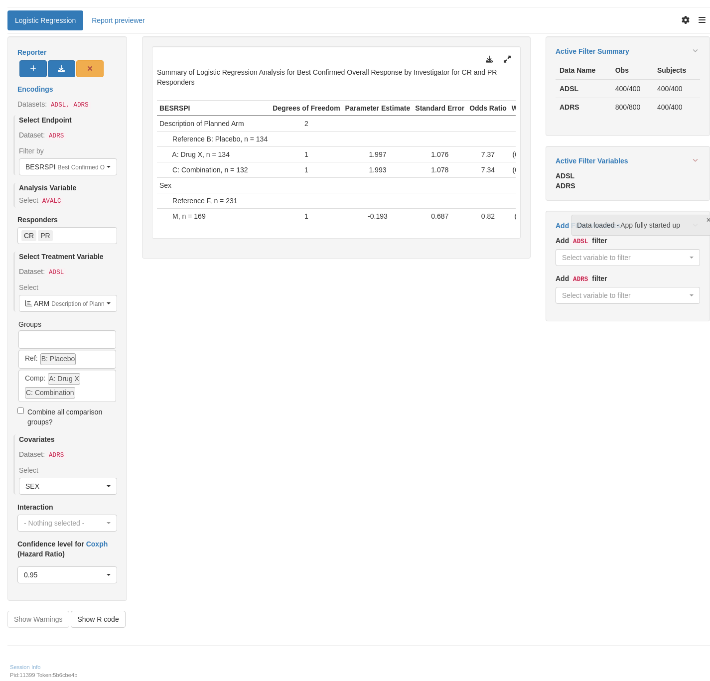
subtitle: Multi-Variable Logistic Regression
---

------------------------------------------------------------------------

{{< include ../../_utils/envir_hook.qmd >}}

```{r setup, echo = FALSE, warning = FALSE, message = FALSE}
library(dplyr)
library(tern)

adsl <- random.cdisc.data::cadsl
adrs <- random.cdisc.data::cadrs

# Ensure character variables are converted to factors and empty strings and NAs are explicit missing levels.
adsl <- df_explicit_na(adsl)
adrs <- df_explicit_na(adrs)

adsl <- adsl %>%
  dplyr::filter(SEX %in% c("F", "M"))

adrs <- adrs %>%
  dplyr::filter(PARAMCD == "BESRSPI") %>%
  dplyr::mutate(
    Response = case_when(AVALC %in% c("PR", "CR") ~ 1, TRUE ~ 0),
    SEX = factor(SEX, c("M", "F")),
    RACE = factor(
      RACE,
      levels = c(
        "AMERICAN INDIAN OR ALASKA NATIVE", "ASIAN", "BLACK OR AFRICAN AMERICAN",
        "WHITE", "MULTIPLE", "NATIVE HAWAIIAN OR OTHER PACIFIC ISLANDER"
      )
    )
  ) %>%
  var_relabel(Response = "Response", SEX = "Sex", RACE = "Race")
```

```{r include = FALSE}
webr_code_labels <- c("setup")
```

{{< include ../../_utils/webr_no_include.qmd >}}

## Output

::::::: panel-tabset
## Multi-Variable Logistic Regression

::: {.panel-tabset .nav-justified group="webr"}
## {{< fa regular file-lines sm fw >}} Preview

```{r variant1, test = list(result_v1 = "result")}
model <- fit_logistic(
  adrs,
  variables = list(response = "Response", arm = "ARMCD", covariates = c("SEX", "AGE"))
)
conf_level <- 0.95
df <- broom::tidy(model, conf_level = conf_level)

# empty string flag
df <- df_explicit_na(df, na_level = "_NA_")

result <- basic_table() %>%
  summarize_logistic(
    conf_level = conf_level,
    drop_and_remove_str = "_NA_"
  ) %>%
  append_topleft("Logistic regression") %>%
  build_table(df = df)
result
```

```{r include = FALSE}
webr_code_labels <- c("variant1")
```

{{< include ../../_utils/webr.qmd >}}
:::

## Multi-Variable Logistic Regression <br/> with Interaction Term

::: {.panel-tabset .nav-justified group="webr"}
## {{< fa regular file-lines sm fw >}} Preview

```{r variant2, test = list(result_v2 = "result")}
model <- fit_logistic(
  adrs,
  variables = list(
    response = "Response",
    arm = "ARMCD",
    covariates = c("SEX", "AGE"),
    interaction = "SEX"
  )
)
conf_level <- 0.95
df <- broom::tidy(model, conf_level = conf_level)

# empty string flag
df <- df_explicit_na(df, na_level = "_NA_")

result <- basic_table() %>%
  summarize_logistic(
    conf_level = conf_level,
    drop_and_remove_str = "_NA_"
  ) %>%
  append_topleft("Logistic regression with interaction") %>%
  build_table(df = df)
result
```

```{r include = FALSE}
webr_code_labels <- c("variant2")
```

{{< include ../../_utils/webr.qmd >}}
:::

## Multi-Variable Logistic Regression <br/> Specifying Covariates

::: {.panel-tabset .nav-justified group="webr"}
## {{< fa regular file-lines sm fw >}} Preview

```{r variant3, test = list(result_v3 = "result")}
model <- fit_logistic(
  adrs,
  variables = list(
    response = "Response",
    arm = "ARMCD",
    covariates = c("SEX", "AGE", "RACE")
  )
)
conf_level <- 0.95
df <- broom::tidy(model, conf_level = conf_level)

# empty string flag
df <- df_explicit_na(df, na_level = "_NA_")

result <- basic_table() %>%
  summarize_logistic(
    conf_level = conf_level,
    drop_and_remove_str = "_NA_"
  ) %>%
  append_topleft("y ~ ARM + SEX + AGE + RACE") %>%
  build_table(df = df)
result
```

```{r include = FALSE}
webr_code_labels <- c("variant3")
```

{{< include ../../_utils/webr.qmd >}}
:::

## Multi-Variable Logistic Regression Setting <br/> an Event, Alpha Level, and Level for Interaction

::: {.panel-tabset .nav-justified group="webr"}
## {{< fa regular file-lines sm fw >}} Preview

```{r variant4, test = list(result_v4 = "result")}
model <- fit_logistic(
  adrs,
  variables = list(
    response = "Response",
    arm = "ARMCD",
    covariates = c("SEX", "AGE"),
    interaction = "AGE"
  ),
  response_definition = "1 - response"
)
conf_level <- 0.9
df <- broom::tidy(model, conf_level = conf_level, at = c(30, 50))

# empty string flag
df <- df_explicit_na(df, na_level = "_NA_")

result <- basic_table() %>%
  summarize_logistic(
    conf_level = conf_level,
    drop_and_remove_str = "_NA_"
  ) %>%
  append_topleft("Estimations at age 30 and 50") %>%
  build_table(df = df)
result
```

```{r include = FALSE}
webr_code_labels <- c("variant4")
```

{{< include ../../_utils/webr.qmd >}}
:::

## Data Setup

```{r setup}
#| code-fold: show
```
:::::::

{{< include ../../_utils/save_results.qmd >}}

## `teal` App

::: {.panel-tabset .nav-justified}
## {{< fa regular file-lines fa-sm fa-fw >}} Preview

```{r teal, opts.label = c("skip_if_testing", "app")}
library(teal.modules.clinical)

## Data reproducible code
data <- teal_data()
data <- within(data, {
  library(dplyr)

  ADSL <- random.cdisc.data::cadsl
  ADRS <- random.cdisc.data::cadrs %>%
    filter(PARAMCD %in% c("BESRSPI", "INVET"))
})
datanames <- c("ADSL", "ADRS")
datanames(data) <- datanames
join_keys(data) <- default_cdisc_join_keys[datanames]

## Reusable Configuration For Modules
ADRS <- data[["ADRS"]]
arm_ref_comp <- list(
  ACTARMCD = list(
    ref = "ARM B",
    comp = c("ARM A", "ARM C")
  ),
  ARM = list(
    ref = "B: Placebo",
    comp = c("A: Drug X", "C: Combination")
  )
)

## Setup App
app <- init(
  data = data,
  modules = modules(
    tm_t_logistic(
      label = "Logistic Regression",
      dataname = "ADRS",
      arm_var = choices_selected(
        choices = variable_choices(ADRS, c("ARM", "ARMCD")),
        selected = "ARM"
      ),
      arm_ref_comp = arm_ref_comp,
      paramcd = choices_selected(
        choices = value_choices(ADRS, "PARAMCD", "PARAM"),
        selected = "BESRSPI"
      ),
      cov_var = choices_selected(
        choices = c("SEX", "AGE", "BMRKR1", "BMRKR2"),
        selected = "SEX"
      )
    )
  )
)

shinyApp(app$ui, app$server)
```

{{< include ../../_utils/shinylive.qmd >}}
:::

{{< include ../../repro.qmd >}}

Made with ❤️ by the NEST Team

  • Edit this page
  • Report an issue
Cookie Preferences