TLG Catalog - Stable
  • Stable
    • Dev
  1. Tables
  2. Lab Results
  3. LBT03
  • Introduction

  • Tables
    • ADA
      • ADAT01
      • ADAT02
      • ADAT03
      • ADAT04A
      • ADAT04B
    • Adverse Events
      • AET01
      • AET01_AESI
      • AET02
      • AET02_SMQ
      • AET03
      • AET04
      • AET04_PI
      • AET05
      • AET05_ALL
      • AET06
      • AET06_SMQ
      • AET07
      • AET09
      • AET09_SMQ
      • AET10
    • Concomitant Medications
      • CMT01
      • CMT01A
      • CMT01B
      • CMT02_PT
    • Deaths
      • DTHT01
    • Demography
      • DMT01
    • Disclosures
      • DISCLOSUREST01
      • EUDRAT01
      • EUDRAT02
    • Disposition
      • DST01
      • PDT01
      • PDT02
    • ECG
      • EGT01
      • EGT02
      • EGT03
      • EGT04
      • EGT05_QTCAT
    • Efficacy
      • AOVT01
      • AOVT02
      • AOVT03
      • CFBT01
      • CMHT01
      • COXT01
      • COXT02
      • DORT01
      • LGRT02
      • MMRMT01
      • ONCT05
      • RATET01
      • RBMIT01
      • RSPT01
      • TTET01
    • Exposure
      • EXT01
    • Lab Results
      • LBT01
      • LBT02
      • LBT03
      • LBT04
      • LBT05
      • LBT06
      • LBT07
      • LBT08
      • LBT09
      • LBT10
      • LBT10_BL
      • LBT11
      • LBT11_BL
      • LBT12
      • LBT12_BL
      • LBT13
      • LBT14
      • LBT15
    • Medical History
      • MHT01
    • Pharmacokinetic
      • PKCT01
      • PKPT02
      • PKPT03
      • PKPT04
      • PKPT05
      • PKPT06
      • PKPT07
      • PKPT08
      • PKPT11
    • Risk Management Plan
      • RMPT01
      • RMPT03
      • RMPT04
      • RMPT05
      • RMPT06
    • Safety
      • ENTXX
    • Vital Signs
      • VST01
      • VST02
  • Listings
    • ADA
      • ADAL02
    • Adverse Events
      • AEL01
      • AEL01_NOLLT
      • AEL02
      • AEL02_ED
      • AEL03
      • AEL04
    • Concomitant Medications
      • CML01
      • CML02A_GL
      • CML02B_GL
    • Development Safety Update Report
      • DSUR4
    • Disposition
      • DSL01
      • DSL02
    • ECG
      • EGL01
    • Efficacy
      • ONCL01
    • Exposure
      • EXL01
    • Lab Results
      • LBL01
      • LBL01_RLS
      • LBL02A
      • LBL02A_RLS
      • LBL02B
    • Medical History
      • MHL01
    • Pharmacokinetic
      • ADAL01
      • PKCL01
      • PKCL02
      • PKPL01
      • PKPL02
      • PKPL04
    • Vital Signs
      • VSL01
  • Graphs
    • Efficacy
      • FSTG01
      • FSTG02
      • KMG01
      • MMRMG01
      • MMRMG02
    • Other
      • BRG01
      • BWG01
      • CIG01
      • IPPG01
      • LTG01
      • MNG01
    • Pharmacokinetic
      • PKCG01
      • PKCG02
      • PKCG03
      • PKPG01
      • PKPG02
      • PKPG03
      • PKPG04
      • PKPG06

  • Appendix
    • Reproducibility

  • Index

On this page

  • Output
  • teal App
  • Reproducibility
    • Timestamp
    • Session Info
    • .lock file
  • Edit this page
  • Report an issue
  1. Tables
  2. Lab Results
  3. LBT03

LBT03

Laboratory Test Results Change from Baseline by Visit


Output

  • Standard Table
  • Data Setup

The LBT03 template is the result of a junction between the analysis of AVAL at baseline and CHG at visit time. AVAL is summarized for baseline visits and and CHG is summarized for post-baseline visits.

  • Preview
  • Try this using WebR
Code
# Define the split function
split_fun <- drop_split_levels

lyt <- basic_table(show_colcounts = TRUE) %>%
  split_cols_by("ARM") %>%
  split_rows_by("AVISIT", split_fun = split_fun, label_pos = "topleft", split_label = obj_label(adlb_f$AVISIT)) %>%
  summarize_change(
    "CHG",
    variables = list(value = "AVAL", baseline_flag = "ABLFLL"),
    na.rm = TRUE
  )

result <- build_table(
  lyt = lyt,
  df = adlb_f,
  alt_counts_df = adsl
)

result
                  A: Drug X      B: Placebo    C: Combination
Analysis Visit     (N=134)        (N=134)         (N=132)    
—————————————————————————————————————————————————————————————
BASELINE                                                     
  n                  134            134             132      
  Mean (SD)      9.06 (0.93)    8.99 (0.98)     8.98 (0.89)  
  Median             9.07           8.92            8.96     
  Min - Max      6.21 - 11.87   6.23 - 11.63    6.24 - 11.18 
WEEK 1 DAY 8                                                 
  n                  134             0              132      
  Mean (SD)      -0.05 (1.38)        NA         -0.02 (1.30) 
  Median            -0.17            NA             0.02     
  Min - Max      -3.56 - 3.48        NA         -3.28 - 3.33 
WEEK 2 DAY 15                                                
  n                  134            134             132      
  Mean (SD)      -0.19 (1.47)   0.01 (1.45)     0.15 (1.25)  
  Median            -0.27          -0.00            0.15     
  Min - Max      -4.53 - 4.45   -3.79 - 3.43    -2.92 - 3.28 
WEEK 3 DAY 22                                                
  n                  134            134             132      
  Mean (SD)      0.03 (1.38)    -0.02 (1.49)    0.02 (1.34)  
  Median             0.15          -0.04            0.20     
  Min - Max      -3.95 - 2.99   -4.28 - 4.24    -2.76 - 3.26 
WEEK 4 DAY 29                                                
  n                  134            134             132      
  Mean (SD)      -0.26 (1.45)   0.05 (1.24)     -0.01 (1.17) 
  Median            -0.37           0.10           -0.06     
  Min - Max      -3.74 - 4.15   -3.34 - 3.71    -3.06 - 3.22 
WEEK 5 DAY 36                                                
  n                  134            134             132      
  Mean (SD)      -0.02 (1.50)   0.07 (1.34)     0.03 (1.27)  
  Median             0.01           0.15            0.05     
  Min - Max      -4.15 - 3.96   -3.50 - 3.53    -3.63 - 4.78 
Experimental use!

WebR is a tool allowing you to run R code in the web browser. Modify the code below and click run to see the results. Alternatively, copy the code and click here to open WebR in a new tab.

In the final step, a new variable is derived from AVISIT that can specify the method of estimation of the evaluated change.

  • Preview
  • Try this using WebR
Code
adlb_f <- adlb_f %>% mutate(AVISIT_header = recode(AVISIT,
  "BASELINE" = "BASELINE",
  "WEEK 1 DAY 8" = "WEEK 1 DAY 8 value minus baseline",
  "WEEK 2 DAY 15" = "WEEK 2 DAY 15 value minus baseline",
  "WEEK 3 DAY 22" = "WEEK 3 DAY 22 value minus baseline",
  "WEEK 4 DAY 29" = "WEEK 4 DAY 29 value minus baseline",
  "WEEK 5 DAY 36" = "WEEK 5 DAY 36 value minus baseline"
))

# Define the split function
split_fun <- drop_split_levels

lyt <- basic_table(show_colcounts = TRUE) %>%
  split_cols_by("ARM") %>%
  split_rows_by("AVISIT_header",
    split_fun = split_fun,
    label_pos = "topleft",
    split_label = obj_label(adlb_f$AVISIT)
  ) %>%
  summarize_change(
    "CHG",
    variables = list(value = "AVAL", baseline_flag = "ABLFLL"),
    na.rm = TRUE
  )

result <- build_table(
  lyt = lyt,
  df = adlb_f,
  alt_counts_df = adsl
)

result
                                      A: Drug X      B: Placebo    C: Combination
Analysis Visit                         (N=134)        (N=134)         (N=132)    
—————————————————————————————————————————————————————————————————————————————————
BASELINE                                                                         
  n                                      134            134             132      
  Mean (SD)                          9.06 (0.93)    8.99 (0.98)     8.98 (0.89)  
  Median                                 9.07           8.92            8.96     
  Min - Max                          6.21 - 11.87   6.23 - 11.63    6.24 - 11.18 
WEEK 1 DAY 8 value minus baseline                                                
  n                                      134             0              132      
  Mean (SD)                          -0.05 (1.38)        NA         -0.02 (1.30) 
  Median                                -0.17            NA             0.02     
  Min - Max                          -3.56 - 3.48        NA         -3.28 - 3.33 
WEEK 2 DAY 15 value minus baseline                                               
  n                                      134            134             132      
  Mean (SD)                          -0.19 (1.47)   0.01 (1.45)     0.15 (1.25)  
  Median                                -0.27          -0.00            0.15     
  Min - Max                          -4.53 - 4.45   -3.79 - 3.43    -2.92 - 3.28 
WEEK 3 DAY 22 value minus baseline                                               
  n                                      134            134             132      
  Mean (SD)                          0.03 (1.38)    -0.02 (1.49)    0.02 (1.34)  
  Median                                 0.15          -0.04            0.20     
  Min - Max                          -3.95 - 2.99   -4.28 - 4.24    -2.76 - 3.26 
WEEK 4 DAY 29 value minus baseline                                               
  n                                      134            134             132      
  Mean (SD)                          -0.26 (1.45)   0.05 (1.24)     -0.01 (1.17) 
  Median                                -0.37           0.10           -0.06     
  Min - Max                          -3.74 - 4.15   -3.34 - 3.71    -3.06 - 3.22 
WEEK 5 DAY 36 value minus baseline                                               
  n                                      134            134             132      
  Mean (SD)                          -0.02 (1.50)   0.07 (1.34)     0.03 (1.27)  
  Median                                 0.01           0.15            0.05     
  Min - Max                          -4.15 - 3.96   -3.50 - 3.53    -3.63 - 4.78 
Experimental use!

WebR is a tool allowing you to run R code in the web browser. Modify the code below and click run to see the results. Alternatively, copy the code and click here to open WebR in a new tab.

For illustration purposes, this example focuses on “C-Reactive Protein Measurement” starting from baseline, while excluding visit at week 1 for subjects who were randomized to the placebo group.

Code
library(dplyr)
library(tern)

adsl <- random.cdisc.data::cadsl
adlb <- random.cdisc.data::cadlb

# Ensure character variables are converted to factors and empty strings and NAs are explicit missing levels.
adsl <- df_explicit_na(adsl)
adlb <- df_explicit_na(adlb)

saved_labels <- var_labels(adlb)

adlb_f <- adlb %>%
  filter(
    PARAM == "C-Reactive Protein Measurement",
    !(ARM == "B: Placebo" & AVISIT == "WEEK 1 DAY 8"),
    AVISIT != "SCREENING"
  ) %>%
  dplyr::mutate(
    AVISIT = droplevels(AVISIT),
    ABLFLL = ABLFL == "Y"
  )

var_labels(adlb_f) <- c(saved_labels, "")

teal App

  • Preview
  • Try this using shinylive

Here, we pre-process and manually define the variable “Baseline or Absolute Change from Baseline”.

Code
library(teal.modules.clinical)

## Data reproducible code
data <- teal_data()
data <- within(data, {
  ADSL <- df_explicit_na(random.cdisc.data::cadsl)
  ADLB <- df_explicit_na(random.cdisc.data::cadlb) %>%
    filter(
      !(ARM == "B: Placebo" & AVISIT == "WEEK 1 DAY 8"),
      AVISIT != "SCREENING"
    ) %>%
    mutate(
      AVISIT = droplevels(AVISIT),
      ABLFLL = ABLFL == "Y",
      AVISIT_header = recode(AVISIT,
        "BASELINE" = "BASELINE",
        "WEEK 1 DAY 8" = "WEEK 1 DAY 8 value minus baseline",
        "WEEK 2 DAY 15" = "WEEK 2 DAY 15 value minus baseline",
        "WEEK 3 DAY 22" = "WEEK 3 DAY 22 value minus baseline",
        "WEEK 4 DAY 29" = "WEEK 4 DAY 29 value minus baseline",
        "WEEK 5 DAY 36" = "WEEK 5 DAY 36 value minus baseline"
      )
    ) %>%
    group_by(USUBJID, PARAM) %>%
    mutate(
      AVAL_CHG = AVAL - (!ABLFLL) * sum(AVAL * ABLFLL)
    ) %>%
    ungroup() %>%
    col_relabel(
      AVAL_CHG = "Baseline or Absolute Change from Baseline",
      ABLFLL = "Baseline Flag (TRUE/FALSE)",
      AVISIT_header = "Analysis Visit"
    )
})
datanames <- c("ADSL", "ADLB")
datanames(data) <- datanames
Warning: `datanames<-()` was deprecated in teal.data 0.7.0.
ℹ invalid to use `datanames()<-` or `names()<-` on an object of class
  `teal_data`. See ?names.teal_data
Code
join_keys(data) <- default_cdisc_join_keys[datanames]

## Reusable Configuration For Modules
ADSL <- data[["ADSL"]]
ADLB <- data[["ADLB"]]

## Setup App
app <- init(
  data = data,
  modules = modules(
    tm_t_summary_by(
      label = "Laboratory Test Results Change from Baseline by Visit",
      dataname = "ADLB",
      arm_var = choices_selected(
        choices = variable_choices(ADSL, c("ARM", "ARMCD")),
        selected = "ARM"
      ),
      by_vars = choices_selected(
        # note: order matters here. If `PARAM` is first, the split will be first by `PARAM`and then by `AVISIT`
        choices = variable_choices(ADLB, c("PARAM", "AVISIT_header")),
        selected = c("PARAM", "AVISIT_header")
      ),
      summarize_vars = choices_selected(
        choices = variable_choices(ADLB, c("AVAL", "CHG", "AVAL_CHG")),
        selected = c("AVAL_CHG")
      ),
      useNA = "ifany",
      paramcd = choices_selected(
        choices = value_choices(ADLB, "PARAMCD", "PARAM"),
        selected = "CRP"
      )
    )
  ),
  filter = teal_slices(teal_slice("ADLB", "AVAL", selected = NULL))
)
shinyApp(app$ui, app$server)

Experimental use!

shinylive allow you to modify to run shiny application entirely in the web browser. Modify the code below and click re-run the app to see the results. The performance is slighly worse and some of the features (e.g. downloading) might not work at all.

#| '!! shinylive warning !!': |
#|   shinylive does not work in self-contained HTML documents.
#|   Please set `embed-resources: false` in your metadata.
#| standalone: true
#| viewerHeight: 800
#| editorHeight: 200
#| components: [viewer, editor]
#| layout: vertical

# -- WEBR HELPERS --
options(webr_pkg_repos = c("r-universe" = "https://insightsengineering.r-universe.dev", getOption("webr_pkg_repos")))

# -- APP CODE --
library(teal.modules.clinical)

## Data reproducible code
data <- teal_data()
data <- within(data, {
  ADSL <- df_explicit_na(random.cdisc.data::cadsl)
  ADLB <- df_explicit_na(random.cdisc.data::cadlb) %>%
    filter(
      !(ARM == "B: Placebo" & AVISIT == "WEEK 1 DAY 8"),
      AVISIT != "SCREENING"
    ) %>%
    mutate(
      AVISIT = droplevels(AVISIT),
      ABLFLL = ABLFL == "Y",
      AVISIT_header = recode(AVISIT,
        "BASELINE" = "BASELINE",
        "WEEK 1 DAY 8" = "WEEK 1 DAY 8 value minus baseline",
        "WEEK 2 DAY 15" = "WEEK 2 DAY 15 value minus baseline",
        "WEEK 3 DAY 22" = "WEEK 3 DAY 22 value minus baseline",
        "WEEK 4 DAY 29" = "WEEK 4 DAY 29 value minus baseline",
        "WEEK 5 DAY 36" = "WEEK 5 DAY 36 value minus baseline"
      )
    ) %>%
    group_by(USUBJID, PARAM) %>%
    mutate(
      AVAL_CHG = AVAL - (!ABLFLL) * sum(AVAL * ABLFLL)
    ) %>%
    ungroup() %>%
    col_relabel(
      AVAL_CHG = "Baseline or Absolute Change from Baseline",
      ABLFLL = "Baseline Flag (TRUE/FALSE)",
      AVISIT_header = "Analysis Visit"
    )
})
datanames <- c("ADSL", "ADLB")
datanames(data) <- datanames
join_keys(data) <- default_cdisc_join_keys[datanames]

## Reusable Configuration For Modules
ADSL <- data[["ADSL"]]
ADLB <- data[["ADLB"]]

## Setup App
app <- init(
  data = data,
  modules = modules(
    tm_t_summary_by(
      label = "Laboratory Test Results Change from Baseline by Visit",
      dataname = "ADLB",
      arm_var = choices_selected(
        choices = variable_choices(ADSL, c("ARM", "ARMCD")),
        selected = "ARM"
      ),
      by_vars = choices_selected(
        # note: order matters here. If `PARAM` is first, the split will be first by `PARAM`and then by `AVISIT`
        choices = variable_choices(ADLB, c("PARAM", "AVISIT_header")),
        selected = c("PARAM", "AVISIT_header")
      ),
      summarize_vars = choices_selected(
        choices = variable_choices(ADLB, c("AVAL", "CHG", "AVAL_CHG")),
        selected = c("AVAL_CHG")
      ),
      useNA = "ifany",
      paramcd = choices_selected(
        choices = value_choices(ADLB, "PARAMCD", "PARAM"),
        selected = "CRP"
      )
    )
  ),
  filter = teal_slices(teal_slice("ADLB", "AVAL", selected = NULL))
)
shinyApp(app$ui, app$server)

Reproducibility

Timestamp

[1] "2025-07-05 17:48:07 UTC"

Session Info

─ Session info ───────────────────────────────────────────────────────────────
 setting  value
 version  R version 4.5.0 (2025-04-11)
 os       Ubuntu 24.04.2 LTS
 system   x86_64, linux-gnu
 ui       X11
 language (EN)
 collate  en_US.UTF-8
 ctype    en_US.UTF-8
 tz       Etc/UTC
 date     2025-07-05
 pandoc   3.7.0.2 @ /usr/bin/ (via rmarkdown)
 quarto   1.7.32 @ /usr/local/bin/quarto

─ Packages ───────────────────────────────────────────────────────────────────
 package               * version  date (UTC) lib source
 backports               1.5.0    2024-05-23 [1] RSPM
 brio                    1.1.5    2024-04-24 [1] RSPM
 broom                   1.0.8    2025-03-28 [1] RSPM
 bslib                   0.9.0    2025-01-30 [1] RSPM
 cachem                  1.1.0    2024-05-16 [1] RSPM
 callr                   3.7.6    2024-03-25 [1] RSPM
 checkmate               2.3.2    2024-07-29 [1] RSPM
 chromote                0.5.1    2025-04-24 [1] RSPM
 cli                     3.6.5    2025-04-23 [1] RSPM
 coda                    0.19-4.1 2024-01-31 [1] CRAN (R 4.5.0)
 codetools               0.2-20   2024-03-31 [2] CRAN (R 4.5.0)
 curl                    6.4.0    2025-06-22 [1] RSPM
 data.table              1.17.6   2025-06-17 [1] RSPM
 dichromat               2.0-0.1  2022-05-02 [1] CRAN (R 4.5.0)
 digest                  0.6.37   2024-08-19 [1] RSPM
 dplyr                 * 1.1.4    2023-11-17 [1] RSPM
 emmeans                 1.11.1   2025-05-04 [1] RSPM
 estimability            1.5.1    2024-05-12 [1] RSPM
 evaluate                1.0.4    2025-06-18 [1] RSPM
 farver                  2.1.2    2024-05-13 [1] RSPM
 fastmap                 1.2.0    2024-05-15 [1] RSPM
 fontawesome             0.5.3    2024-11-16 [1] RSPM
 forcats                 1.0.0    2023-01-29 [1] RSPM
 formatR                 1.14     2023-01-17 [1] CRAN (R 4.5.0)
 formatters            * 0.5.11   2025-04-09 [1] RSPM
 geepack                 1.3.12   2024-09-23 [1] RSPM
 generics                0.1.4    2025-05-09 [1] RSPM
 ggplot2                 3.5.2    2025-04-09 [1] RSPM
 glue                    1.8.0    2024-09-30 [1] RSPM
 gtable                  0.3.6    2024-10-25 [1] RSPM
 htmltools               0.5.8.1  2024-04-04 [1] RSPM
 htmlwidgets             1.6.4    2023-12-06 [1] RSPM
 httpuv                  1.6.16   2025-04-16 [1] RSPM
 httr                    1.4.7    2023-08-15 [1] RSPM
 jquerylib               0.1.4    2021-04-26 [1] RSPM
 jsonlite                2.0.0    2025-03-27 [1] RSPM
 knitr                   1.50     2025-03-16 [1] RSPM
 later                   1.4.2    2025-04-08 [1] RSPM
 lattice                 0.22-7   2025-04-02 [2] CRAN (R 4.5.0)
 lazyeval                0.2.2    2019-03-15 [1] RSPM
 lifecycle               1.0.4    2023-11-07 [1] RSPM
 logger                  0.4.0    2024-10-22 [1] RSPM
 magrittr              * 2.0.3    2022-03-30 [1] RSPM
 MASS                    7.3-65   2025-02-28 [2] CRAN (R 4.5.0)
 Matrix                  1.7-3    2025-03-11 [1] CRAN (R 4.5.0)
 memoise                 2.0.1    2021-11-26 [1] RSPM
 mime                    0.13     2025-03-17 [1] RSPM
 multcomp                1.4-28   2025-01-29 [1] RSPM
 mvtnorm                 1.3-3    2025-01-10 [1] RSPM
 nestcolor               0.1.3    2025-01-21 [1] RSPM
 nlme                    3.1-168  2025-03-31 [2] CRAN (R 4.5.0)
 pillar                  1.11.0   2025-07-04 [1] RSPM
 pkgcache                2.2.4    2025-05-26 [1] RSPM
 pkgconfig               2.0.3    2019-09-22 [1] RSPM
 plotly                  4.11.0   2025-06-19 [1] RSPM
 processx                3.8.6    2025-02-21 [1] RSPM
 promises                1.3.3    2025-05-29 [1] RSPM
 ps                      1.9.1    2025-04-12 [1] RSPM
 purrr                   1.0.4    2025-02-05 [1] RSPM
 R6                      2.6.1    2025-02-15 [1] RSPM
 random.cdisc.data       0.3.16   2024-10-10 [1] RSPM
 rbibutils               2.3      2024-10-04 [1] RSPM
 RColorBrewer            1.1-3    2022-04-03 [1] RSPM
 Rcpp                    1.1.0    2025-07-02 [1] RSPM
 Rdpack                  2.6.4    2025-04-09 [1] RSPM
 rlang                   1.1.6    2025-04-11 [1] RSPM
 rmarkdown               2.29     2024-11-04 [1] RSPM
 rtables               * 0.6.13   2025-06-19 [1] RSPM
 sandwich                3.1-1    2024-09-15 [1] RSPM
 sass                    0.4.10   2025-04-11 [1] RSPM
 scales                  1.4.0    2025-04-24 [1] RSPM
 sessioninfo             1.2.3    2025-02-05 [1] any (@1.2.3)
 shiny                 * 1.11.1   2025-07-03 [1] RSPM
 shinycssloaders         1.1.0    2024-07-30 [1] RSPM
 shinyjs                 2.1.0    2021-12-23 [1] RSPM
 shinyvalidate           0.1.3    2023-10-04 [1] RSPM
 shinyWidgets            0.9.0    2025-02-21 [1] RSPM
 stringi                 1.8.7    2025-03-27 [1] RSPM
 stringr                 1.5.1    2023-11-14 [1] RSPM
 survival                3.8-3    2024-12-17 [2] CRAN (R 4.5.0)
 teal                  * 0.16.0   2025-02-23 [1] RSPM
 teal.code             * 0.6.1    2025-02-14 [1] RSPM
 teal.data             * 0.7.0    2025-01-28 [1] RSPM
 teal.logger             0.3.2    2025-02-14 [1] RSPM
 teal.modules.clinical * 0.10.0   2025-02-28 [1] RSPM
 teal.reporter           0.4.0    2025-01-24 [1] RSPM
 teal.slice            * 0.6.0    2025-02-03 [1] RSPM
 teal.transform        * 0.6.0    2025-02-12 [1] RSPM
 teal.widgets            0.4.3    2025-01-31 [1] RSPM
 tern                  * 0.9.9    2025-06-20 [1] RSPM
 tern.gee                0.1.5    2024-08-23 [1] RSPM
 testthat                3.2.3    2025-01-13 [1] RSPM
 TH.data                 1.1-3    2025-01-17 [1] RSPM
 tibble                  3.3.0    2025-06-08 [1] RSPM
 tidyr                   1.3.1    2024-01-24 [1] RSPM
 tidyselect              1.2.1    2024-03-11 [1] RSPM
 vctrs                   0.6.5    2023-12-01 [1] RSPM
 viridisLite             0.4.2    2023-05-02 [1] RSPM
 webshot                 0.5.5    2023-06-26 [1] CRAN (R 4.5.0)
 webshot2                0.1.2    2025-04-23 [1] RSPM
 websocket               1.4.4    2025-04-10 [1] RSPM
 withr                   3.0.2    2024-10-28 [1] RSPM
 xfun                    0.52     2025-04-02 [1] RSPM
 xtable                  1.8-4    2019-04-21 [1] RSPM
 yaml                    2.3.10   2024-07-26 [1] RSPM
 zoo                     1.8-14   2025-04-10 [1] RSPM

 [1] /usr/local/lib/R/site-library
 [2] /usr/local/lib/R/library
 [3] /github/home/R/x86_64-pc-linux-gnu-library/4.5
 * ── Packages attached to the search path.

──────────────────────────────────────────────────────────────────────────────

.lock file

Download the .lock file and use renv::restore() on it to recreate environment used to generate this website.

Download

LBT02
LBT04
Source Code
---
title: LBT03
subtitle: Laboratory Test Results Change from Baseline by Visit
---

------------------------------------------------------------------------

{{< include ../../_utils/envir_hook.qmd >}}

```{r setup, echo = FALSE, warning = FALSE, message = FALSE}
library(dplyr)
library(tern)

adsl <- random.cdisc.data::cadsl
adlb <- random.cdisc.data::cadlb

# Ensure character variables are converted to factors and empty strings and NAs are explicit missing levels.
adsl <- df_explicit_na(adsl)
adlb <- df_explicit_na(adlb)

saved_labels <- var_labels(adlb)

adlb_f <- adlb %>%
  filter(
    PARAM == "C-Reactive Protein Measurement",
    !(ARM == "B: Placebo" & AVISIT == "WEEK 1 DAY 8"),
    AVISIT != "SCREENING"
  ) %>%
  dplyr::mutate(
    AVISIT = droplevels(AVISIT),
    ABLFLL = ABLFL == "Y"
  )

var_labels(adlb_f) <- c(saved_labels, "")
```

```{r include = FALSE}
webr_code_labels <- c("setup")
```

{{< include ../../_utils/webr_no_include.qmd >}}

## Output

::::: panel-tabset
## Standard Table

The `LBT03` template is the result of a junction between the analysis of `AVAL` at baseline and `CHG` at visit time. `AVAL` is summarized for baseline visits and and `CHG` is summarized for post-baseline visits.

::: {.panel-tabset .nav-justified group="webr"}
## {{< fa regular file-lines sm fw >}} Preview

```{r variant1, test = list(result_v1 = "result")}
# Define the split function
split_fun <- drop_split_levels

lyt <- basic_table(show_colcounts = TRUE) %>%
  split_cols_by("ARM") %>%
  split_rows_by("AVISIT", split_fun = split_fun, label_pos = "topleft", split_label = obj_label(adlb_f$AVISIT)) %>%
  summarize_change(
    "CHG",
    variables = list(value = "AVAL", baseline_flag = "ABLFLL"),
    na.rm = TRUE
  )

result <- build_table(
  lyt = lyt,
  df = adlb_f,
  alt_counts_df = adsl
)

result
```

```{r include = FALSE}
webr_code_labels <- c("variant1")
```

{{< include ../../_utils/webr.qmd >}}
:::

In the final step, a new variable is derived from `AVISIT` that can specify the method of estimation of the evaluated change.

::: {.panel-tabset .nav-justified group="webr"}
## {{< fa regular file-lines sm fw >}} Preview

```{r variant2, test = list(result_v2 = "result")}
adlb_f <- adlb_f %>% mutate(AVISIT_header = recode(AVISIT,
  "BASELINE" = "BASELINE",
  "WEEK 1 DAY 8" = "WEEK 1 DAY 8 value minus baseline",
  "WEEK 2 DAY 15" = "WEEK 2 DAY 15 value minus baseline",
  "WEEK 3 DAY 22" = "WEEK 3 DAY 22 value minus baseline",
  "WEEK 4 DAY 29" = "WEEK 4 DAY 29 value minus baseline",
  "WEEK 5 DAY 36" = "WEEK 5 DAY 36 value minus baseline"
))

# Define the split function
split_fun <- drop_split_levels

lyt <- basic_table(show_colcounts = TRUE) %>%
  split_cols_by("ARM") %>%
  split_rows_by("AVISIT_header",
    split_fun = split_fun,
    label_pos = "topleft",
    split_label = obj_label(adlb_f$AVISIT)
  ) %>%
  summarize_change(
    "CHG",
    variables = list(value = "AVAL", baseline_flag = "ABLFLL"),
    na.rm = TRUE
  )

result <- build_table(
  lyt = lyt,
  df = adlb_f,
  alt_counts_df = adsl
)

result
```

```{r include = FALSE}
webr_code_labels <- c("variant2")
```

{{< include ../../_utils/webr.qmd >}}
:::

## Data Setup

For illustration purposes, this example focuses on "C-Reactive Protein Measurement" starting from baseline, while excluding visit at week 1 for subjects who were randomized to the placebo group.

```{r setup}
#| code-fold: show
```
:::::

{{< include ../../_utils/save_results.qmd >}}
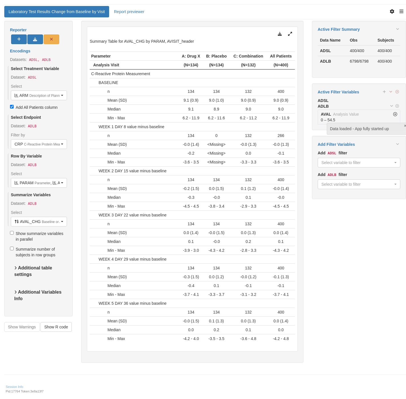
## `teal` App

::: {.panel-tabset .nav-justified}
## {{< fa regular file-lines fa-sm fa-fw >}} Preview

Here, we pre-process and manually define the variable "Baseline or Absolute Change from Baseline".

```{r teal, opts.label = c("skip_if_testing", "app")}
library(teal.modules.clinical)

## Data reproducible code
data <- teal_data()
data <- within(data, {
  ADSL <- df_explicit_na(random.cdisc.data::cadsl)
  ADLB <- df_explicit_na(random.cdisc.data::cadlb) %>%
    filter(
      !(ARM == "B: Placebo" & AVISIT == "WEEK 1 DAY 8"),
      AVISIT != "SCREENING"
    ) %>%
    mutate(
      AVISIT = droplevels(AVISIT),
      ABLFLL = ABLFL == "Y",
      AVISIT_header = recode(AVISIT,
        "BASELINE" = "BASELINE",
        "WEEK 1 DAY 8" = "WEEK 1 DAY 8 value minus baseline",
        "WEEK 2 DAY 15" = "WEEK 2 DAY 15 value minus baseline",
        "WEEK 3 DAY 22" = "WEEK 3 DAY 22 value minus baseline",
        "WEEK 4 DAY 29" = "WEEK 4 DAY 29 value minus baseline",
        "WEEK 5 DAY 36" = "WEEK 5 DAY 36 value minus baseline"
      )
    ) %>%
    group_by(USUBJID, PARAM) %>%
    mutate(
      AVAL_CHG = AVAL - (!ABLFLL) * sum(AVAL * ABLFLL)
    ) %>%
    ungroup() %>%
    col_relabel(
      AVAL_CHG = "Baseline or Absolute Change from Baseline",
      ABLFLL = "Baseline Flag (TRUE/FALSE)",
      AVISIT_header = "Analysis Visit"
    )
})
datanames <- c("ADSL", "ADLB")
datanames(data) <- datanames
join_keys(data) <- default_cdisc_join_keys[datanames]

## Reusable Configuration For Modules
ADSL <- data[["ADSL"]]
ADLB <- data[["ADLB"]]

## Setup App
app <- init(
  data = data,
  modules = modules(
    tm_t_summary_by(
      label = "Laboratory Test Results Change from Baseline by Visit",
      dataname = "ADLB",
      arm_var = choices_selected(
        choices = variable_choices(ADSL, c("ARM", "ARMCD")),
        selected = "ARM"
      ),
      by_vars = choices_selected(
        # note: order matters here. If `PARAM` is first, the split will be first by `PARAM`and then by `AVISIT`
        choices = variable_choices(ADLB, c("PARAM", "AVISIT_header")),
        selected = c("PARAM", "AVISIT_header")
      ),
      summarize_vars = choices_selected(
        choices = variable_choices(ADLB, c("AVAL", "CHG", "AVAL_CHG")),
        selected = c("AVAL_CHG")
      ),
      useNA = "ifany",
      paramcd = choices_selected(
        choices = value_choices(ADLB, "PARAMCD", "PARAM"),
        selected = "CRP"
      )
    )
  ),
  filter = teal_slices(teal_slice("ADLB", "AVAL", selected = NULL))
)
shinyApp(app$ui, app$server)
```

{{< include ../../_utils/shinylive.qmd >}}
:::

{{< include ../../repro.qmd >}}

Made with ❤️ by the NEST Team

  • Edit this page
  • Report an issue
Cookie Preferences