---
title: CIG01
subtitle: Confidence Interval Plot
---
------------------------------------------------------------------------
{{< include ../../_utils/envir_hook.qmd >}}
```{r setup, echo = FALSE, warning = FALSE, message = FALSE}
library(tern)
library(ggplot2)
library(dplyr)
library(nestcolor)
adlb <- random.cdisc.data::cadlb %>%
filter(PARAMCD == "ALT", AVISIT == "BASELINE")
```
```{r include = FALSE}
webr_code_labels <- c("setup")
```
{{< include ../../_utils/webr_no_include.qmd >}}
## Output
:::::::: panel-tabset
## Plot of Mean and <br/> 95% CIs for Mean
::: {.panel-tabset .nav-justified group="webr"}
## {{< fa regular file-lines sm fw >}} Preview
The function `stat_mean_ci` from the `tern` package can be used with default values to draw the 95% confidence interval around the mean.
```{r plot1and2, test = list(plot_v1_and_v2 = "plot")}
plot <- ggplot(
  data = adlb,
  mapping = aes(
    x = ARMCD, y = AVAL, color = SEX,
    lty = SEX, shape = SEX
  )
) +
  stat_summary(
    fun.data = tern::stat_mean_ci,
    geom = "errorbar",
    width = 0.1,
    position = position_dodge(width = 0.5)
  ) +
  stat_summary(
    fun = mean,
    geom = "point",
    position = position_dodge(width = 0.5)
  ) +
  labs(
    title = "Confidence Interval Plot by Treatment Group",
    caption = "Mean and 95% CIs for mean are displayed.",
    x = "Treatment Group",
    y = paste0(adlb$PARAMCD[1], " (", adlb$AVALU[1], ")")
  )
plot
```
```{r include = FALSE}
webr_code_labels <- c("plot1and2")
```
{{< include ../../_utils/webr.qmd >}}
:::
## Plot of Confidence Interval Using <br/> a Different Stratification Variable
::: {.panel-tabset .nav-justified group="webr"}
## {{< fa regular file-lines sm fw >}} Preview
```{r plot3, test = list(plot_v3 = "plot")}
plot <- ggplot(
  data = adlb,
  mapping = aes(
    x = ARMCD, y = AVAL, color = STRATA2,
    lty = STRATA2, shape = STRATA2
  )
) +
  stat_summary(
    fun.data = tern::stat_mean_ci,
    geom = "errorbar",
    width = 0.1,
    position = position_dodge(width = 0.5)
  ) +
  stat_summary(
    fun = mean,
    geom = "point",
    position = position_dodge(width = 0.5)
  ) +
  labs(
    title = "Confidence Interval Plot by Treatment Group",
    caption = "Mean and 95% CIs for mean are displayed.",
    x = "Treatment Group",
    y = paste0(adlb$PARAMCD[1], " (", adlb$AVALU[1], ")")
  )
plot
```
```{r include = FALSE}
webr_code_labels <- c("plot3")
```
{{< include ../../_utils/webr.qmd >}}
:::
## Plot of Median and <br/> 95% CIs for Median
::: {.panel-tabset .nav-justified group="webr"}
## {{< fa regular file-lines sm fw >}} Preview
The function `stat_median_ci` from the `tern` package works similarly to `stat_mean_ci`.
```{r plot4, test = list(plot_v4 = "plot")}
plot <- ggplot(
  data = adlb,
  mapping = aes(
    x = ARMCD, y = AVAL, color = STRATA1,
    lty = STRATA1, shape = STRATA1
  )
) +
  stat_summary(
    fun.data = stat_median_ci,
    geom = "errorbar",
    width = 0.1,
    position = position_dodge(width = 0.5)
  ) +
  stat_summary(
    fun = median,
    geom = "point",
    position = position_dodge(width = 0.5)
  ) +
  labs(
    title = "Confidence Interval Plot by Treatment Group",
    caption = "Median and 95% CIs for median are displayed.",
    x = "Treatment Group",
    y = paste0(adlb$PARAMCD[1], " (", adlb$AVALU[1], ")")
  )
plot
```
```{r include = FALSE}
webr_code_labels <- c("plot4")
```
{{< include ../../_utils/webr.qmd >}}
:::
## Plot of Median and 95% CIs for <br/> Median Using Different Alpha Level
::: {.panel-tabset .nav-justified group="webr"}
## {{< fa regular file-lines sm fw >}} Preview
To modify the confidence level for the estimation of the confidence interval, the call to `stat_mean_ci` (or `stat_median_ci`) can be slightly modified.
```{r plot5, test = list(plot_v5 = "plot")}
plot <- ggplot(
  data = adlb,
  mapping = aes(
    x = ARMCD, y = AVAL, color = SEX,
    lty = SEX, shape = SEX
  )
) +
  stat_summary(
    fun.data = function(x) tern::stat_mean_ci(x, conf_level = 0.9),
    geom = "errorbar",
    width = 0.1,
    position = position_dodge(width = 0.5)
  ) +
  stat_summary(
    fun = mean,
    geom = "point",
    position = position_dodge(width = 0.5)
  ) +
  labs(
    title = "Confidence Interval Plot by Treatment Group",
    caption = "Mean and 90% CIs for mean are displayed.",
    x = "Treatment Group",
    y = paste0(adlb$PARAMCD[1], " (", adlb$AVALU[1], ")")
  )
plot
```
```{r include = FALSE}
webr_code_labels <- c("plot5")
```
{{< include ../../_utils/webr.qmd >}}
:::
## Table of Mean <br/> and Median
::: {.panel-tabset .nav-justified group="webr"}
## {{< fa regular file-lines sm fw >}} Preview
The corresponding table is simply obtained using the `rtables` framework:
```{r table6, test = list(table_v6 = "table")}
lyt <- basic_table() %>%
  split_cols_by(var = "ARMCD") %>%
  analyze_vars(vars = "AVAL", .stats = c("mean_sd", "median"))
table <- build_table(lyt = lyt, df = adlb)
table
```
```{r include = FALSE}
webr_code_labels <- c("table6")
```
{{< include ../../_utils/webr.qmd >}}
:::
## Data Setup
```{r setup}
#| code-fold: show
```
::::::::
{{< include ../../_utils/save_results.qmd >}}
## `teal` App
::: {.panel-tabset .nav-justified}
## {{< fa regular file-lines fa-sm fa-fw >}} Preview
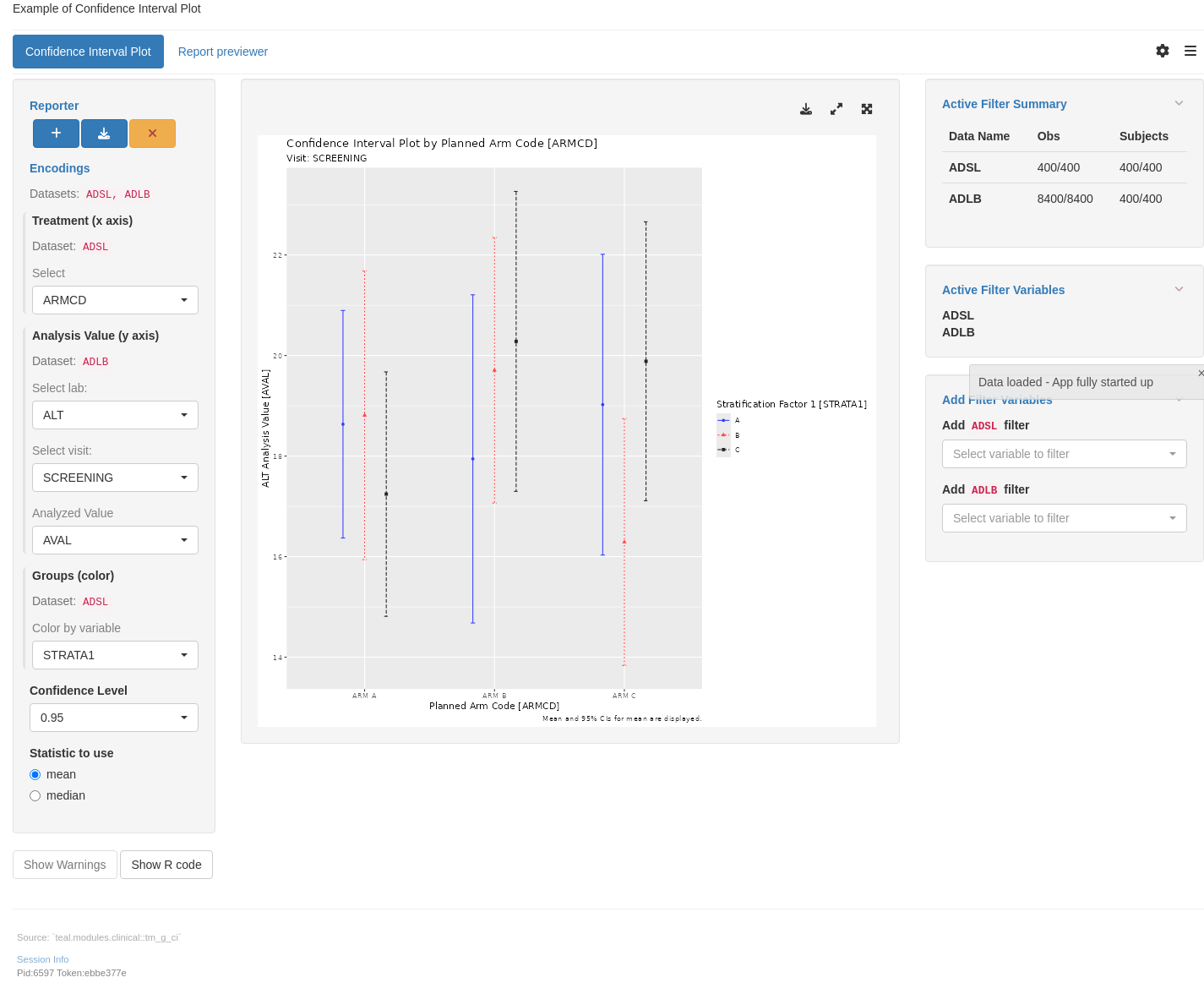
```{r teal, opts.label = c("skip_if_testing", "app")}
library(teal.modules.clinical)

## Data reproducible code
data <- teal_data()
data <- within(data, {
  ADSL <- random.cdisc.data::cadsl
  ADLB <- random.cdisc.data::cadlb
})
join_keys(data) <- default_cdisc_join_keys[c("ADSL", "ADLB")]

## Reusable Configuration For Modules
ADLB <- data[["ADLB"]]

## Setup App
app <- init(
  data = data,
  modules = modules(
    tm_g_ci(
      label = "Confidence Interval Plot",
      x_var = data_extract_spec(
        dataname = "ADSL",
        select = select_spec(
          choices = c("ARMCD", "BMRKR2"),
          selected = c("ARMCD"),
          multiple = FALSE,
          fixed = FALSE
        )
      ),
      y_var = data_extract_spec(
        dataname = "ADLB",
        filter = list(
          filter_spec(
            vars = "PARAMCD",
            choices = levels(ADLB$PARAMCD),
            selected = levels(ADLB$PARAMCD)[1],
            multiple = FALSE,
            label = "Select lab:"
          ),
          filter_spec(
            vars = "AVISIT",
            choices = levels(ADLB$AVISIT),
            selected = levels(ADLB$AVISIT)[1],
            multiple = FALSE,
            label = "Select visit:"
          )
        ),
        select = select_spec(
          label = "Analyzed Value",
          choices = c("AVAL", "CHG"),
          selected = "AVAL",
          multiple = FALSE,
          fixed = FALSE
        )
      ),
      color = data_extract_spec(
        dataname = "ADSL",
        select = select_spec(
          label = "Color by variable",
          choices = c("SEX", "STRATA1", "STRATA2"),
          selected = c("STRATA1"),
          multiple = FALSE,
          fixed = FALSE
        )
      )
    )
  ),
  header = "Example of Confidence Interval Plot",
  footer = tags$p(
    class = "text-muted", "Source: `teal.modules.clinical::tm_g_ci`"
  )
)
shinyApp(app$ui, app$server)
```
{{< include ../../_utils/shinylive.qmd >}}
:::
{{< include ../../repro.qmd >}}