SPG2

STEP Graphs for Response Outcome

SPG

We will use the cadrs data set from the random.cdisc.data package to create the STEP response graph. We start by filtering the adrs data set for response evaluable patients and the response parameter of interest, creating a new logical variable encoding response (response patients should solely be CR patients), binarizing the ARM variable.

Code

library(tern)
library(ggplot2.utils)
library(dplyr)

adrs <- random.cdisc.data::cadrs %>%
  df_explicit_na() %>%
  filter(PARAM == "Best Confirmed Overall Response by Investigator", BMEASIFL == "Y") %>%
  mutate(
    is_rsp = AVALC == "CR",
    ARM_BIN = fct_collapse_only(
      ARM,
      CTRL = c("B: Placebo"),
      TRT = c("A: Drug X", "C: Combination")
    )
  )

We then perform with the fit_rsp_step() function the required calculations: this function fits the Subgroup Treatment Effect Pattern (STEP) logistic regression models for the response outcome within each of the percentile intervals of the age variable AGE defining the subgroups. The treatment arm variable must have exactly two levels, where the first one is taken as reference, i.e. the estimated odds ratios are for the comparison of the second level vs. the first one.

In this example we fit the default model where a constant treatment effect is estimated in each of the subgroups that are created according to age quantiles.

Code

vars <- list(
  time = "AVAL",
  response = "is_rsp",
  arm = "ARM_BIN",
  biomarker = "AGE"
)

step_matrix <- fit_rsp_step(
  variables = vars,
  data = adrs
)

In this second example we fit instead a model with a linear age interaction term and we control the bandwidth (50% of data) of the STEP windows for the age variable.

Code

step_matrix <- fit_rsp_step(
  variables = vars,
  data = adrs,
  control = c(control_logistic(), control_step(degree = 1, bandwidth = 0.5))
)

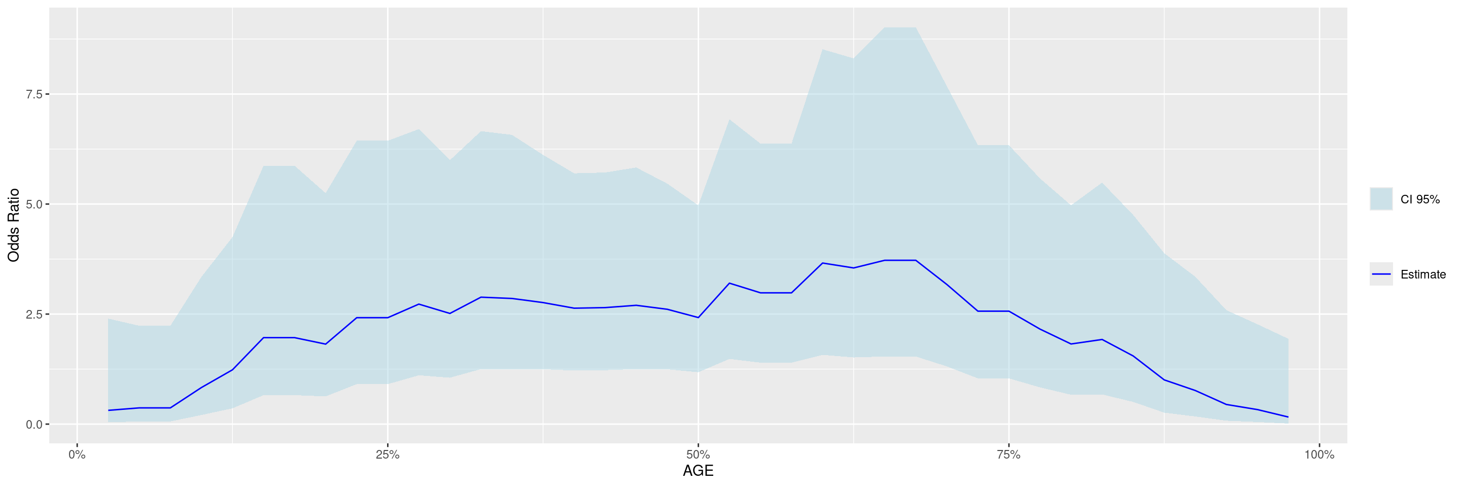
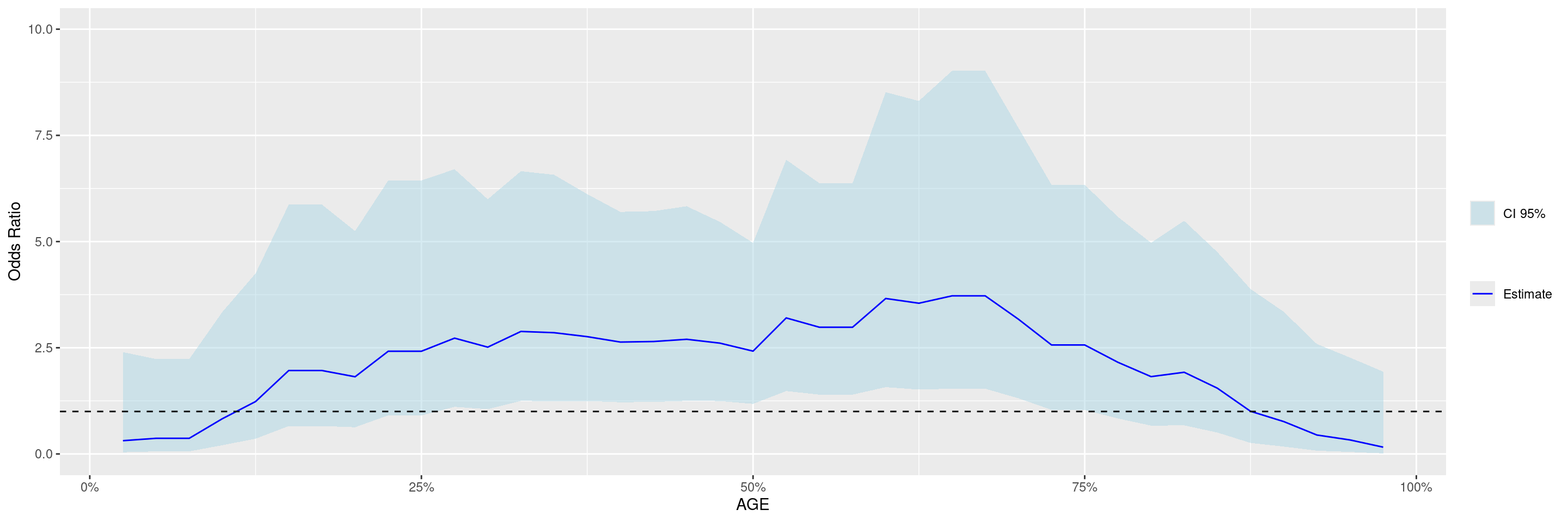
Before we can plot the data, the broom::tidy() method needs to be applied to the STEP result to obtain graph ready data. Thereafter with the g_step() function we can create a graph showing the estimated odds ratio along the continuous age subgroups.

Code

step_data <- broom::tidy(step_matrix)

graph <- g_step(step_data)

graph

We can also add a reference line and change the axis limits.

Code

graph +
  geom_hline(aes(yintercept = 1), linetype = 2) +
  coord_cartesian(ylim = c(0, 10))

Code

sessionInfo()

R version 4.4.2 (2024-10-31)
Platform: x86_64-pc-linux-gnu
Running under: Ubuntu 24.04.1 LTS

Matrix products: default
BLAS:   /usr/lib/x86_64-linux-gnu/openblas-pthread/libblas.so.3 
LAPACK: /usr/lib/x86_64-linux-gnu/openblas-pthread/libopenblasp-r0.3.26.so;  LAPACK version 3.12.0

locale:
 [1] LC_CTYPE=en_US.UTF-8       LC_NUMERIC=C              
 [3] LC_TIME=en_US.UTF-8        LC_COLLATE=en_US.UTF-8    
 [5] LC_MONETARY=en_US.UTF-8    LC_MESSAGES=en_US.UTF-8   
 [7] LC_PAPER=en_US.UTF-8       LC_NAME=C                 
 [9] LC_ADDRESS=C               LC_TELEPHONE=C            
[11] LC_MEASUREMENT=en_US.UTF-8 LC_IDENTIFICATION=C       

time zone: Etc/UTC
tzcode source: system (glibc)

attached base packages:
[1] stats     graphics  grDevices utils     datasets  methods   base     

other attached packages:
[1] dplyr_1.1.4         ggplot2.utils_0.3.2 ggplot2_3.5.1      
[4] tern_0.9.7          rtables_0.6.11      magrittr_2.0.3     
[7] formatters_0.5.10  

loaded via a namespace (and not attached):
 [1] generics_0.1.3           tidyr_1.3.1              EnvStats_3.0.0          
 [4] stringi_1.8.4            lattice_0.22-6           digest_0.6.37           
 [7] evaluate_1.0.3           grid_4.4.2               fastmap_1.2.0           
[10] jsonlite_1.9.0           Matrix_1.7-2             backports_1.5.0         
[13] survival_3.8-3           purrr_1.0.4              scales_1.3.0            
[16] codetools_0.2-20         Rdpack_2.6.2             cli_3.6.4               
[19] ggpp_0.5.8-1             nestcolor_0.1.3          rlang_1.1.5             
[22] rbibutils_2.3            munsell_0.5.1            splines_4.4.2           
[25] withr_3.0.2              yaml_2.3.10              tools_4.4.2             
[28] polynom_1.4-1            checkmate_2.3.2          colorspace_2.1-1        
[31] forcats_1.0.0            ggstats_0.8.0            broom_1.0.7             
[34] vctrs_0.6.5              R6_2.6.1                 lifecycle_1.0.4         
[37] stringr_1.5.1            htmlwidgets_1.6.4        MASS_7.3-64             
[40] pkgconfig_2.0.3          pillar_1.10.1            gtable_0.3.6            
[43] glue_1.8.0               xfun_0.51                tibble_3.2.1            
[46] tidyselect_1.2.1         knitr_1.49               farver_2.1.2            
[49] htmltools_0.5.8.1        labeling_0.4.3           rmarkdown_2.29          
[52] random.cdisc.data_0.3.16 compiler_4.4.2

Reuse