DG1

Histograms of Numeric Variables

We will use the cadsl data set from the random.cdisc.data package and ggplot2 to create the plots. In this example, we will plot histograms of one or multiple numeric variables. We start by selecting the biomarker evaluable population with the flag variable BEP01FL and then populating a new continuous biomarker variable, BMRKR3.

Code

library(tern)
library(ggplot2.utils)
library(dplyr)
library(tibble)
library(tidyr)

adsl <- random.cdisc.data::cadsl %>%
  df_explicit_na() %>%
  filter(BEP01FL == "Y") %>%
  mutate(BMRKR3 = rnorm(n(), mean = 7, sd = 2))

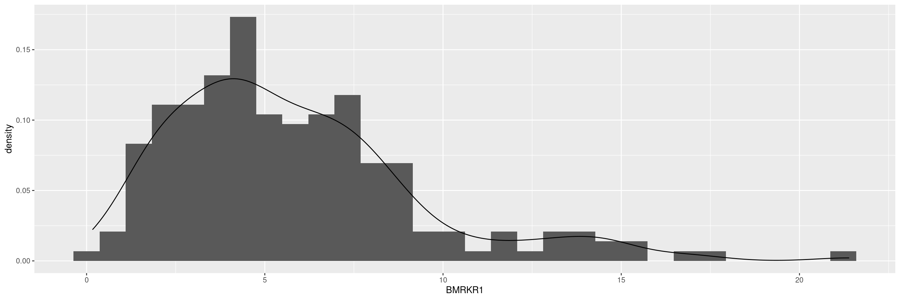
In this example, we will create a combined histogram/density graph of a continuous biomarker variable. Note that you may run into warning messages after producing the graph if the variable you want to analyze contains NAs. To avoid these warning messages, you can use the drop_na() function from tidyr in the data manipulation step above to remove the NAs rows from the dataset (e.g drop_na(BMRKR1)).

Code

graph <- ggplot(adsl, aes(BMRKR1)) +
  geom_histogram(aes(y = after_stat(density)), bins = 30) +
  geom_density(aes(y = after_stat(density)))

graph

We can also calculate some descriptive statistics and populate a table that we can overlay on top of the plot. The tibble function is used to build a data frame data_tb with 3 variables. The x and y variables represent the coordinates on the plot to show the statistic values and can be modified based on preference. For example, x = 1 and y = 1 will put the statistics table in the top right corner of the graph, while x = 0 and y = 0 will put the statistics table in the bottom left corner of the graph. The tb variable contains the statistics to be shown on the plot, in the form of a nested list column starting from the original statistics tibble orig_tb. Finally, we can use the geom_table_npc() layer function to process the data_tb input and add the statistics table to the existing graph.

Code

orig_tb <- with(adsl, tribble(
  ~Statistic, ~Value,
  "N", length(BMRKR1),
  "SD", sd(BMRKR1),
  "Median", median(BMRKR1),
  "Min.", min(BMRKR1),
  "Max.", max(BMRKR1)
))

data_tb <- tibble(x = 1, y = 1, tb = list(orig_tb))

graph <- graph +
  geom_table_npc(data = data_tb, aes(npcx = x, npcy = y, label = tb))

graph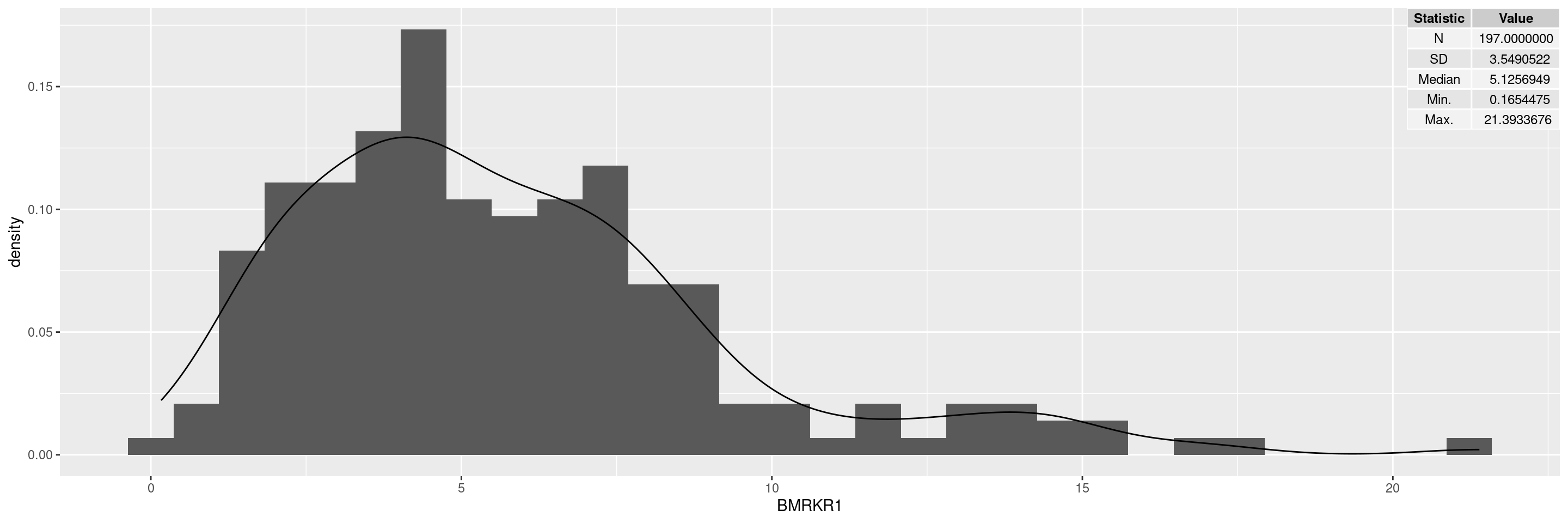

Code

sessionInfo()

R version 4.4.2 (2024-10-31)
Platform: x86_64-pc-linux-gnu
Running under: Ubuntu 24.04.1 LTS

Matrix products: default
BLAS:   /usr/lib/x86_64-linux-gnu/openblas-pthread/libblas.so.3 
LAPACK: /usr/lib/x86_64-linux-gnu/openblas-pthread/libopenblasp-r0.3.26.so;  LAPACK version 3.12.0

locale:
 [1] LC_CTYPE=en_US.UTF-8       LC_NUMERIC=C              
 [3] LC_TIME=en_US.UTF-8        LC_COLLATE=en_US.UTF-8    
 [5] LC_MONETARY=en_US.UTF-8    LC_MESSAGES=en_US.UTF-8   
 [7] LC_PAPER=en_US.UTF-8       LC_NAME=C                 
 [9] LC_ADDRESS=C               LC_TELEPHONE=C            
[11] LC_MEASUREMENT=en_US.UTF-8 LC_IDENTIFICATION=C       

time zone: Etc/UTC
tzcode source: system (glibc)

attached base packages:
[1] stats     graphics  grDevices utils     datasets  methods   base     

other attached packages:
[1] tidyr_1.3.1         tibble_3.2.1        dplyr_1.1.4        
[4] ggplot2.utils_0.3.2 ggplot2_3.5.1       tern_0.9.7         
[7] rtables_0.6.11      magrittr_2.0.3      formatters_0.5.10  

loaded via a namespace (and not attached):
 [1] generics_0.1.3           EnvStats_3.0.0           stringi_1.8.4           
 [4] lattice_0.22-6           digest_0.6.37            evaluate_1.0.3          
 [7] grid_4.4.2               fastmap_1.2.0            jsonlite_1.9.0          
[10] Matrix_1.7-2             backports_1.5.0          survival_3.8-3          
[13] gridExtra_2.3            purrr_1.0.4              scales_1.3.0            
[16] codetools_0.2-20         Rdpack_2.6.2             cli_3.6.4               
[19] ggpp_0.5.8-1             nestcolor_0.1.3          rlang_1.1.5             
[22] rbibutils_2.3            munsell_0.5.1            splines_4.4.2           
[25] withr_3.0.2              yaml_2.3.10              tools_4.4.2             
[28] polynom_1.4-1            checkmate_2.3.2          colorspace_2.1-1        
[31] forcats_1.0.0            ggstats_0.8.0            broom_1.0.7             
[34] vctrs_0.6.5              R6_2.6.1                 lifecycle_1.0.4         
[37] stringr_1.5.1            htmlwidgets_1.6.4        MASS_7.3-64             
[40] pkgconfig_2.0.3          pillar_1.10.1            gtable_0.3.6            
[43] glue_1.8.0               xfun_0.51                tidyselect_1.2.1        
[46] knitr_1.49               farver_2.1.2             htmltools_0.5.8.1       
[49] labeling_0.4.3           rmarkdown_2.29           random.cdisc.data_0.3.16
[52] compiler_4.4.2

Reuse