RNAG3

RNAseq PCA Graphs

RNAG

This page can be used as a template of how to use the available hermes functions for principal components analysis and plots of RNAseq data sets.

The principal components analysis function uses HermesData as input. See RNAG1 for details.

Code

library(hermes)

object <- hermes_data %>%
  add_quality_flags() %>%
  filter() %>%
  normalize()

Once we have filtered out low quality genes and samples, and normalized the counts, we can perform principal components analysis of the gene counts across all samples using the calc_pca() function. The calc_pca() function uses by default the raw counts, unless otherwise specified in the assay_name argument of the function.

Code

result <- calc_pca(object)

result_cpm <- calc_pca(object, assay_name = "cpm")

We can then also plot these principal component results using the corresponding autoplot() method.

Code

autoplot(result)

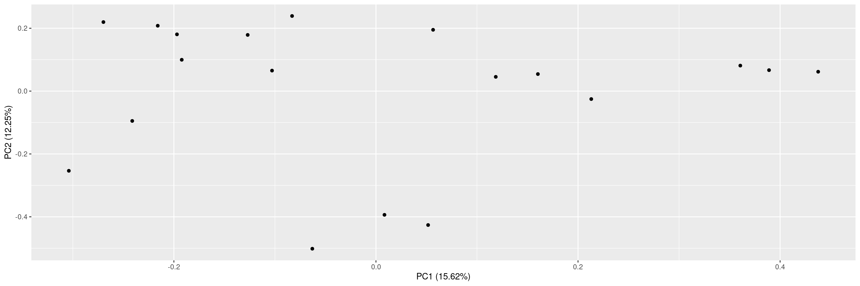
There are many different options for plotting. See ?autoplot.pca_common for the full details. Here some examples.

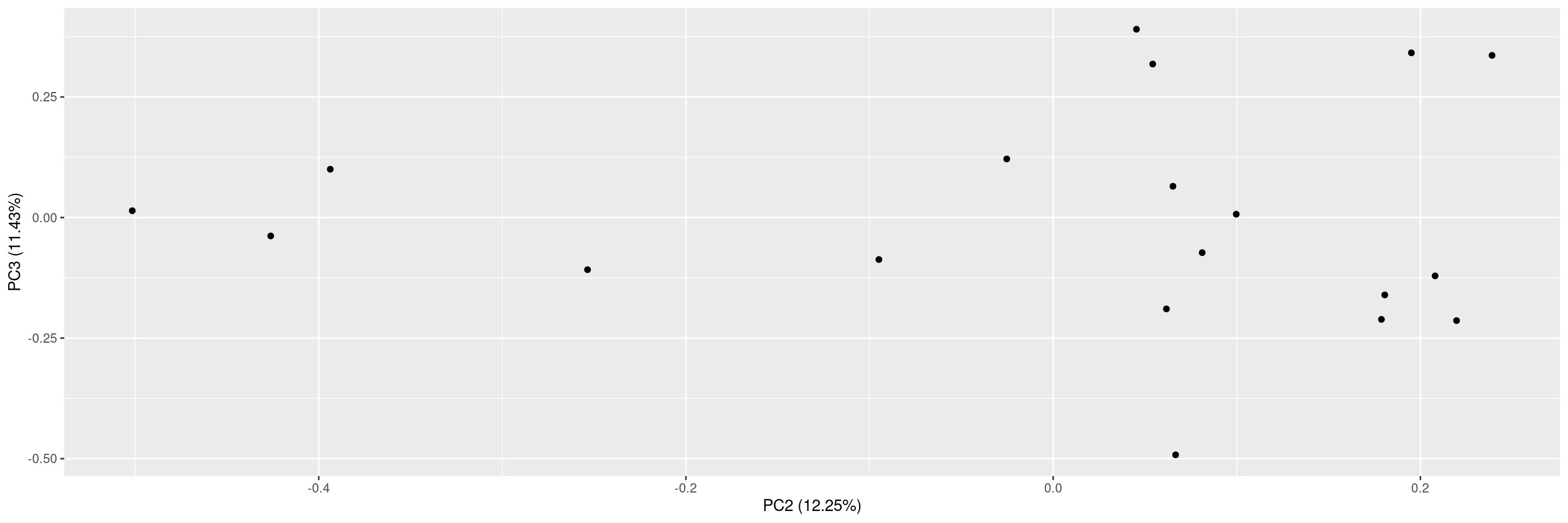
We can specify which principal components should be plotted against each other.

Code

autoplot(result, x = 2, y = 3)

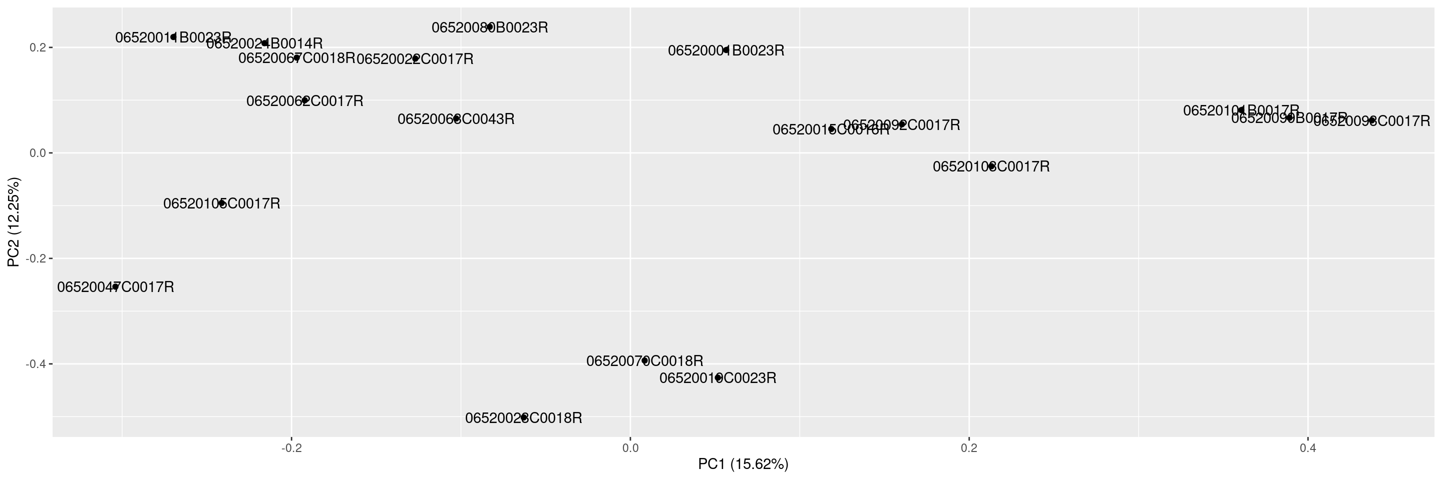
We can also include sample labels on the plot.

Code

autoplot(result, label = TRUE)

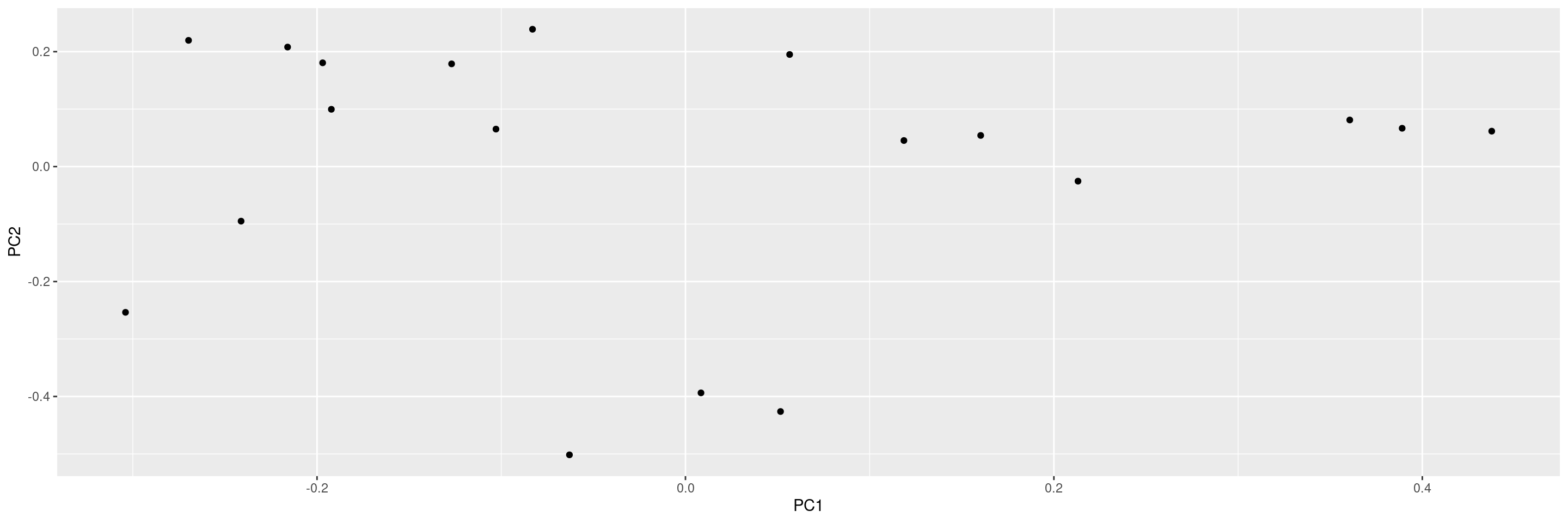
Or we can exclude the variance percentages from the axis labels.

Code

autoplot(result, variance_percentage = FALSE)

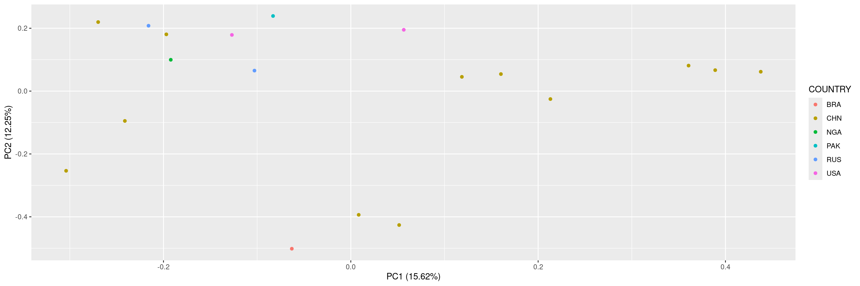
As a last example, we can also color the points by a sample variable.

Code

autoplot(result, data = as.data.frame(colData(object)), colour = "COUNTRY")

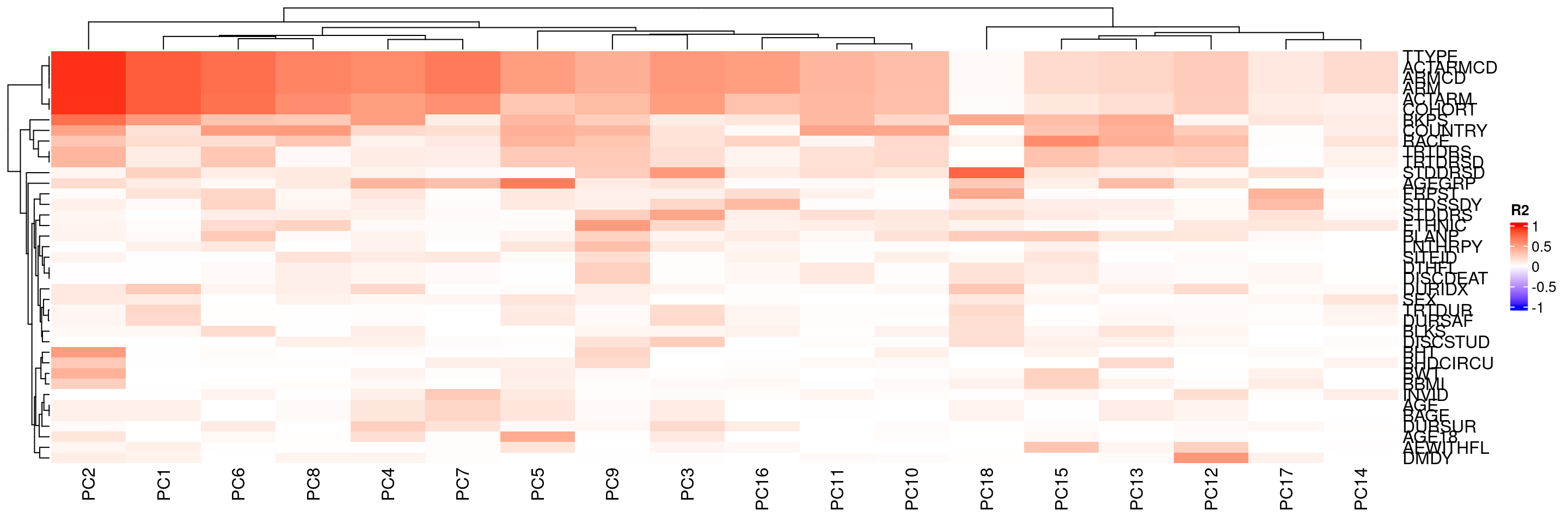
We can also calculate the correlation (in R2 values) between sample variables in HermesData and the principal components of these samples using correlate():

Code

cors <- correlate(result, object)

We can then also plot these R2 values between sample variables and principal components again using the autoplot() method. Sample variables that have high correlation with major principal components can point to potential batch effects.

Code

autoplot(cors)

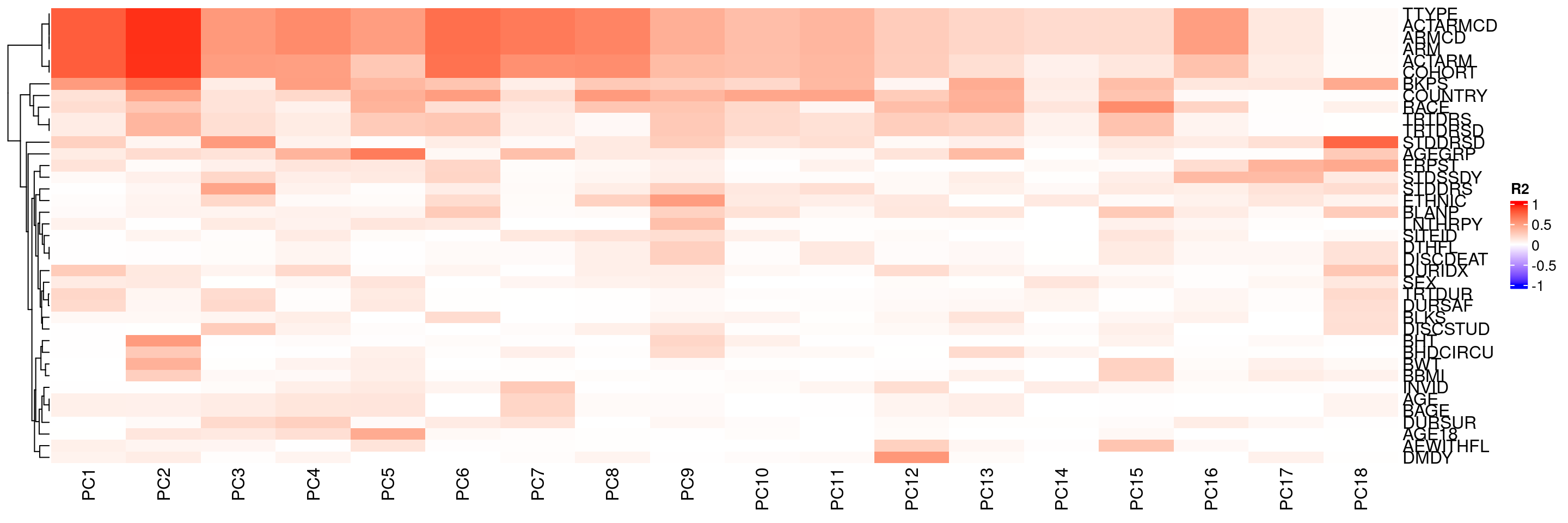
We can also avoid reordering the principal components column.

Code

autoplot(cors, cluster_columns = FALSE)

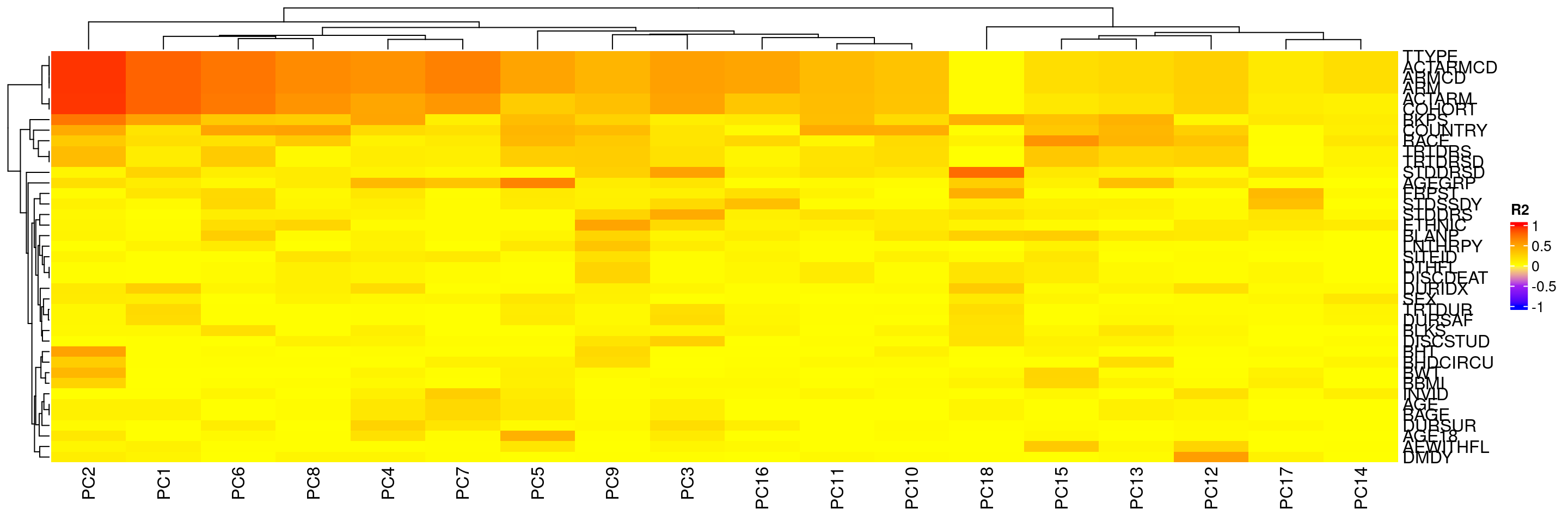
We can also update the color definitions of R2 values in the heatmap.

Code

autoplot(cors,
  cor_colors = circlize::colorRamp2(
    breaks = c(-1, -0.5, 0, 0.5, 1),
    colors = c("blue", "purple", "yellow", "orange", "red")
  )
)

See ?pca_cor_samplevar for the detailed options.

We start by importing a MultiAssayExperiment; here we use the example multi_assay_experiment available in hermes. It is wrapped as a teal::dataset. We can then use the provided teal module tm_g_pca to include a PCA module in our teal app.

Code

library(teal.modules.hermes)

data <- teal_data()
data <- within(data, {
  library(hermes)
  MAE <- multi_assay_experiment
})
datanames(data) <- "MAE"

Warning: `datanames<-()` was deprecated in teal.data 0.7.0.
ℹ invalid to use `datanames()<-` or `names()<-` on an object of class
  `teal_data`. See ?names.teal_data

Code

app <- init(
  data = data,
  modules = modules(
    tm_g_pca(
      label = "pca",
      mae_name = "MAE"
    )
  )
)

[INFO] 2025-02-19 17:29:05.3732 pid:4743 token:[] teal.modules.hermes Initializing tm_g_pca

Code

shinyApp(app$ui, app$server)

Warning: 'experiments' dropped; see 'drops()'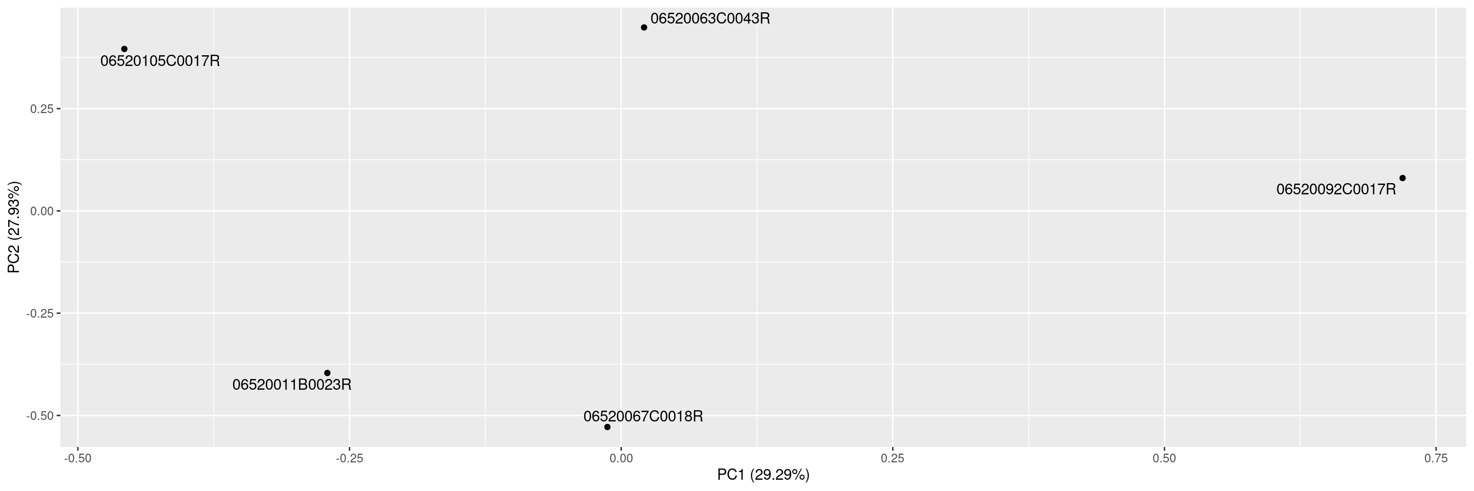

Code

sessionInfo()

R version 4.4.2 (2024-10-31)
Platform: x86_64-pc-linux-gnu
Running under: Ubuntu 24.04.1 LTS

Matrix products: default
BLAS:   /usr/lib/x86_64-linux-gnu/openblas-pthread/libblas.so.3 
LAPACK: /usr/lib/x86_64-linux-gnu/openblas-pthread/libopenblasp-r0.3.26.so;  LAPACK version 3.12.0

locale:
 [1] LC_CTYPE=en_US.UTF-8       LC_NUMERIC=C              
 [3] LC_TIME=en_US.UTF-8        LC_COLLATE=en_US.UTF-8    
 [5] LC_MONETARY=en_US.UTF-8    LC_MESSAGES=en_US.UTF-8   
 [7] LC_PAPER=en_US.UTF-8       LC_NAME=C                 
 [9] LC_ADDRESS=C               LC_TELEPHONE=C            
[11] LC_MEASUREMENT=en_US.UTF-8 LC_IDENTIFICATION=C       

time zone: Etc/UTC
tzcode source: system (glibc)

attached base packages:
[1] stats4    stats     graphics  grDevices utils     datasets  methods  
[8] base     

other attached packages:
 [1] teal.modules.hermes_0.1.6   teal_0.16.0                
 [3] teal.slice_0.6.0            teal.data_0.7.0            
 [5] teal.code_0.6.1             shiny_1.10.0               
 [7] hermes_1.10.0               SummarizedExperiment_1.36.0
 [9] Biobase_2.66.0              GenomicRanges_1.58.0       
[11] GenomeInfoDb_1.42.3         IRanges_2.40.1             
[13] S4Vectors_0.44.0            BiocGenerics_0.52.0        
[15] MatrixGenerics_1.18.1       matrixStats_1.5.0          
[17] ggfortify_0.4.17            ggplot2_3.5.1              

loaded via a namespace (and not attached):
  [1] RColorBrewer_1.1-3          jsonlite_1.9.0             
  [3] shape_1.4.6.1               MultiAssayExperiment_1.32.0
  [5] magrittr_2.0.3              magick_2.8.5               
  [7] farver_2.1.2                rmarkdown_2.29             
  [9] ragg_1.3.3                  GlobalOptions_0.1.2        
 [11] zlibbioc_1.52.0             vctrs_0.6.5                
 [13] memoise_2.0.1               webshot_0.5.5              
 [15] BiocBaseUtils_1.9.0         htmltools_0.5.8.1          
 [17] S4Arrays_1.6.0              forcats_1.0.0              
 [19] progress_1.2.3              curl_6.2.1                 
 [21] SparseArray_1.6.1           sass_0.4.9                 
 [23] bslib_0.9.0                 fontawesome_0.5.3          
 [25] htmlwidgets_1.6.4           testthat_3.2.3             
 [27] httr2_1.1.0                 cachem_1.1.0               
 [29] teal.widgets_0.4.3          mime_0.12                  
 [31] lifecycle_1.0.4             iterators_1.0.14           
 [33] pkgconfig_2.0.3             webshot2_0.1.1             
 [35] Matrix_1.7-2                R6_2.6.1                   
 [37] fastmap_1.2.0               GenomeInfoDbData_1.2.13    
 [39] rbibutils_2.3               clue_0.3-66                
 [41] digest_0.6.37               colorspace_2.1-1           
 [43] shinycssloaders_1.1.0       ps_1.9.0                   
 [45] AnnotationDbi_1.68.0        DESeq2_1.46.0              
 [47] textshaping_1.0.0           crosstalk_1.2.1            
 [49] RSQLite_2.3.9               filelock_1.0.3             
 [51] labeling_0.4.3              httr_1.4.7                 
 [53] abind_1.4-8                 compiler_4.4.2             
 [55] bit64_4.6.0-1               withr_3.0.2                
 [57] doParallel_1.0.17           backports_1.5.0            
 [59] BiocParallel_1.40.0         DBI_1.2.3                  
 [61] logger_0.4.0                biomaRt_2.62.1             
 [63] rappdirs_0.3.3              DelayedArray_0.32.0        
 [65] rjson_0.2.23                tools_4.4.2                
 [67] chromote_0.4.0              httpuv_1.6.15              
 [69] glue_1.8.0                  callr_3.7.6                
 [71] promises_1.3.2              grid_4.4.2                 
 [73] checkmate_2.3.2             cluster_2.1.8              
 [75] generics_0.1.3              gtable_0.3.6               
 [77] websocket_1.4.2             tidyr_1.3.1                
 [79] hms_1.1.3                   xml2_1.3.6                 
 [81] XVector_0.46.0              ggrepel_0.9.6              
 [83] foreach_1.5.2               pillar_1.10.1              
 [85] stringr_1.5.1               limma_3.62.2               
 [87] later_1.4.1                 circlize_0.4.16            
 [89] dplyr_1.1.4                 BiocFileCache_2.14.0       
 [91] lattice_0.22-6              bit_4.5.0.1                
 [93] tidyselect_1.2.1            ComplexHeatmap_2.22.0      
 [95] locfit_1.5-9.11             Biostrings_2.74.1          
 [97] knitr_1.49                  gridExtra_2.3              
 [99] teal.logger_0.3.2           edgeR_4.4.2                
[101] xfun_0.51                   statmod_1.5.0              
[103] brio_1.1.5                  DT_0.33                    
[105] stringi_1.8.4               UCSC.utils_1.2.0           
[107] yaml_2.3.10                 shinyWidgets_0.8.7         
[109] evaluate_1.0.3              codetools_0.2-20           
[111] tibble_3.2.1                cli_3.6.4                  
[113] systemfonts_1.2.1           xtable_1.8-4               
[115] Rdpack_2.6.2                jquerylib_0.1.4            
[117] processx_3.8.5              munsell_0.5.1              
[119] teal.reporter_0.4.0         Rcpp_1.0.14                
[121] dbplyr_2.5.0                png_0.1-8                  
[123] parallel_4.4.2              assertthat_0.2.1           
[125] blob_1.2.4                  prettyunits_1.2.0          
[127] scales_1.3.0                purrr_1.0.4                
[129] crayon_1.5.3                GetoptLong_1.0.5           
[131] rlang_1.1.5                 formatR_1.14               
[133] KEGGREST_1.46.0             shinyjs_2.1.0

Reuse