Biomarker Analysis Catalog - Stable
  • Stable
    • Dev
  1. Graphs
  2. SFG
  3. SFG6
  • Index

  • Tables
    • CPMT
      • CPMT1
      • CPMT2
        • CPMT2A
      • CPMT3
    • DT
      • DT1
        • DT1A
        • DT1B
        • DT1C
      • DT2
        • DT2A
    • TET
      • TET1
        • TET1A

  • Graphs
    • AG
      • AG1
    • DG
      • DG1
        • DG1A
        • DG1B
      • DG2
      • DG3
        • DG3A
      • DG4
    • KG
      • KG1
        • KG1A
        • KG1B
      • KG2
        • KG2A
      • KG3
      • KG4
        • KG4A
        • KG4B
      • KG5
        • KG5A
        • KG5B
    • RFG
      • RFG1
        • RFG1A
      • RFG2
        • RFG2A
        • RFG2B
        • RFG2C
      • RFG3
    • RG
      • RG1
        • RG1A
        • RG1B
        • RG1C
      • RG2
        • RG2A
      • RG3
        • RG3A
        • RG3B
    • SPG
      • SPG1
      • SPG2
    • RNAG
      • RNAG1
      • RNAG2
      • RNAG3
      • RNAG4
      • RNAG5
      • RNAG6
      • RNAG7
      • RNAG8
      • RNAG9
      • RNAG10
    • SFG
      • SFG1
        • SFG1A
        • SFG1B
      • SFG2
        • SFG2A
        • SFG2B
        • SFG2C
        • SFG2D
      • SFG3
        • SFG3A
      • SFG4
      • SFG5
        • SFG5A
        • SFG5B
        • SFG5C
      • SFG6
        • SFG6A
        • SFG6B
        • SFG6C
  1. Graphs
  2. SFG
  3. SFG6

SFG6A

Survival Forest Graph for Multiple Continuous Biomarkers

SFG

  • Setup
  • Plot
  • Session Info

These templates are helpful when we are interested in modelling the effects of continuous biomarker variables on a time-to-event (survival) outcome, conditional on covariates and/or stratification variables included in Cox proportional hazards regression models. We would like to assess how the estimates effects change when we look at different subgroups.

In detail the differences to the other survival forest graphs (SFG1 to SFG5) are the following:

  • The extract_survival_subgroups() and tabulate_survival_subgroups() functions evaluate the treatment effects comparing two arms, across subgroups. On the other hand, the extract_survival_biomarkers() and tabulate_survival_biomarkers() functions used here in SFG6 evaluate the effects from continuous biomarkers in the Cox proportional hazards models, across subgroups.
  • The extract_survival_subgroups() and tabulate_survival_subgroups() functions only allow specification of a single treatment arm variable, while the extract_survival_biomarkers() and tabulate_survival_biomarkers() allow to look at multiple continuous biomarker variables at once.
  • In addition to the treatment arms, the use of extract_survival_subgroups() and tabulate_survival_subgroups() functions can be extended to other binary variables, as done in SFG3 and SFG4. For example, we could define the binarized ARM variable as AGE>=65 vs. AGE<65 and then look at the odds ratios across subgroups. For the extract_survival_biomarkers() and tabulate_survival_biomarkers() functions, we could use the original continuous biomarker variable AGE, and then look at the estimated effect across subgroups.

Similarly like in SFG3, we will use the cadtte data set from the random.cdisc.data package. Here we just filter for the overall survival outcome in a single arm in the biomarker evaluable population.

Code
library(tern)
library(dplyr)

adtte_f <- random.cdisc.data::cadtte %>%
  df_explicit_na() %>%
  filter(
    PARAMCD == "OS",
    ARM == "A: Drug X",
    BEP01FL == "Y"
  ) %>%
  mutate(
    AVAL = day2month(AVAL),
    AVALU = "Months",
    is_event = CNSR == 0
  ) %>%
  var_relabel(
    BEP01FL = "BEP",
    BMRKR1 = "Biomarker (Countinuous)"
  )

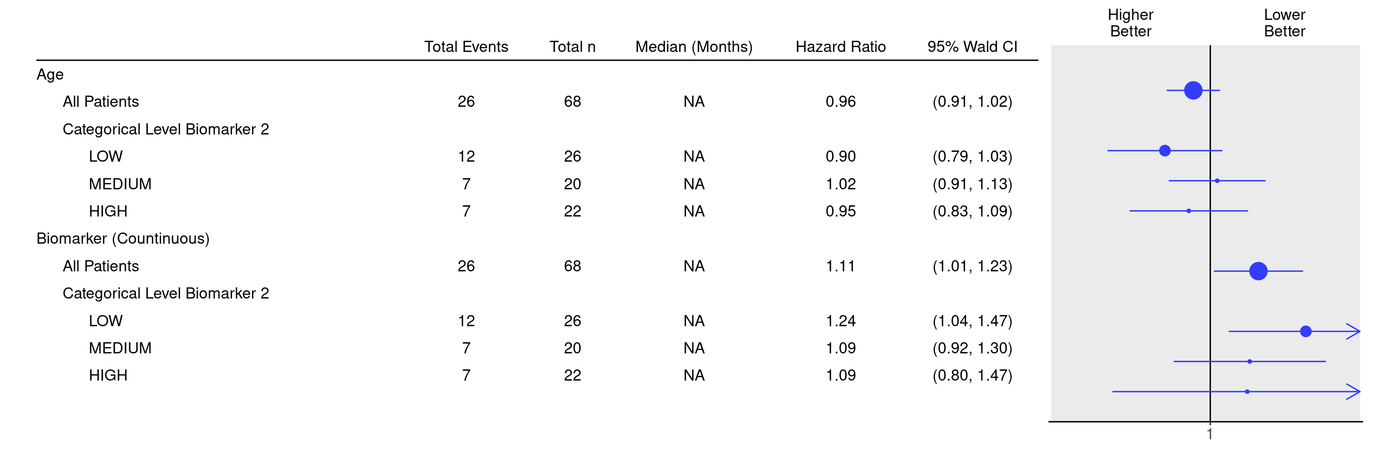
Here we specify that we would like to analyze the two continuous biomarkers BMRKR1 and AGE, conditional on the covariate SEX, in the subgroups defined by the levels of BMRKR2.

Code
df <- extract_survival_biomarkers(
  variables = list(
    tte = "AVAL",
    is_event = "is_event",
    biomarkers = c("BMRKR1", "AGE"),
    covariates = "SEX",
    subgroups = "BMRKR2"
  ),
  data = adtte_f
)

result <- tabulate_survival_biomarkers(
  df = df,
  vars = c("n_tot_events", "n_tot", "median", "hr", "ci"),
  time_unit = adtte_f$AVALU[1]
)

We can look at the result in the console already.

Code
result
                                  Total Events   Total n   Median (Months)   Hazard Ratio   95% Wald CI 
————————————————————————————————————————————————————————————————————————————————————————————————————————
Age                                                                                                     
  All Patients                         26          68            NA              0.96       (0.91, 1.02)
  Categorical Level Biomarker 2                                                                         
    LOW                                12          26            NA              0.90       (0.79, 1.03)
    MEDIUM                             7           20            NA              1.02       (0.91, 1.13)
    HIGH                               7           22            NA              0.95       (0.83, 1.09)
Biomarker (Countinuous)                                                                                 
  All Patients                         26          68            NA              1.11       (1.01, 1.23)
  Categorical Level Biomarker 2                                                                         
    LOW                                12          26            NA              1.24       (1.04, 1.47)
    MEDIUM                             7           20            NA              1.09       (0.92, 1.30)
    HIGH                               7           22            NA              1.09       (0.80, 1.47)

Note that in addition to the Categorical Level Biomarker 2 subgroups we automatically also get the estimates for the overall patient population in the All Patients rows.

We can then produce the final forest plot using the g_forest() function on this tabular result.

Code
g_forest(result, xlim = c(0.7, 1.4))

Here we can see that the continuous biomarker (BMRKR1) shows a trend towards an estimated positive effect on survival (it is not statistically significant though as the confidence intervals still overlap the hazard ratio 1). It is a bit easier to see this here rather than in a cutpoint analysis as presented in SFG3.

Code
sessionInfo()
R version 4.4.2 (2024-10-31)
Platform: x86_64-pc-linux-gnu
Running under: Ubuntu 24.04.1 LTS

Matrix products: default
BLAS:   /usr/lib/x86_64-linux-gnu/openblas-pthread/libblas.so.3 
LAPACK: /usr/lib/x86_64-linux-gnu/openblas-pthread/libopenblasp-r0.3.26.so;  LAPACK version 3.12.0

locale:
 [1] LC_CTYPE=en_US.UTF-8       LC_NUMERIC=C              
 [3] LC_TIME=en_US.UTF-8        LC_COLLATE=en_US.UTF-8    
 [5] LC_MONETARY=en_US.UTF-8    LC_MESSAGES=en_US.UTF-8   
 [7] LC_PAPER=en_US.UTF-8       LC_NAME=C                 
 [9] LC_ADDRESS=C               LC_TELEPHONE=C            
[11] LC_MEASUREMENT=en_US.UTF-8 LC_IDENTIFICATION=C       

time zone: Etc/UTC
tzcode source: system (glibc)

attached base packages:
[1] stats     graphics  grDevices utils     datasets  methods   base     

other attached packages:
[1] dplyr_1.1.4       tern_0.9.7        rtables_0.6.11    magrittr_2.0.3   
[5] formatters_0.5.10

loaded via a namespace (and not attached):
 [1] generics_0.1.3           tidyr_1.3.1              stringi_1.8.4           
 [4] lattice_0.22-6           digest_0.6.37            evaluate_1.0.3          
 [7] grid_4.4.2               fastmap_1.2.0            jsonlite_1.9.0          
[10] Matrix_1.7-2             backports_1.5.0          Formula_1.2-5           
[13] survival_3.8-3           purrr_1.0.4              scales_1.3.0            
[16] codetools_0.2-20         abind_1.4-8              Rdpack_2.6.2            
[19] cli_3.6.4                nestcolor_0.1.3          rlang_1.1.5             
[22] rbibutils_2.3            cowplot_1.1.3            munsell_0.5.1           
[25] splines_4.4.2            withr_3.0.2              yaml_2.3.10             
[28] tools_4.4.2              checkmate_2.3.2          colorspace_2.1-1        
[31] ggplot2_3.5.1            forcats_1.0.0            broom_1.0.7             
[34] vctrs_0.6.5              R6_2.6.1                 lifecycle_1.0.4         
[37] stringr_1.5.1            car_3.1-3                htmlwidgets_1.6.4       
[40] pkgconfig_2.0.3          pillar_1.10.1            gtable_0.3.6            
[43] glue_1.8.0               xfun_0.51                tibble_3.2.1            
[46] tidyselect_1.2.1         knitr_1.49               farver_2.1.2            
[49] htmltools_0.5.8.1        labeling_0.4.3           rmarkdown_2.29          
[52] carData_3.0-5            random.cdisc.data_0.3.16 compiler_4.4.2          

Reuse

Copyright 2023, Hoffmann-La Roche Ltd.
SFG5C
SFG6B
Source Code
---
title: SFG6A
subtitle: Survival Forest Graph for Multiple Continuous Biomarkers
categories: [SFG]
---

------------------------------------------------------------------------

::: panel-tabset
{{< include setup.qmd >}}

## Plot

Here we specify that we would like to analyze the two continuous biomarkers `BMRKR1` and `AGE`, conditional on the covariate `SEX`, in the subgroups defined by the levels of `BMRKR2`.

```{r}
df <- extract_survival_biomarkers(
  variables = list(
    tte = "AVAL",
    is_event = "is_event",
    biomarkers = c("BMRKR1", "AGE"),
    covariates = "SEX",
    subgroups = "BMRKR2"
  ),
  data = adtte_f
)

result <- tabulate_survival_biomarkers(
  df = df,
  vars = c("n_tot_events", "n_tot", "median", "hr", "ci"),
  time_unit = adtte_f$AVALU[1]
)
```

We can look at the result in the console already.

```{r}
result
```

Note that in addition to the `Categorical Level Biomarker 2` subgroups we automatically also get the estimates for the overall patient population in the `All Patients` rows.

We can then produce the final forest plot using the `g_forest()` function on this tabular result.

```{r, fig.width = 15}
g_forest(result, xlim = c(0.7, 1.4))
```

Here we can see that the continuous biomarker (`BMRKR1`) shows a trend towards an estimated positive effect on survival (it is not statistically significant though as the confidence intervals still overlap the hazard ratio 1).
It is a bit easier to see this here rather than in a cutpoint analysis as presented in [SFG3](../../graphs/SFG3/sfg03.qmd).

{{< include ../../misc/session_info.qmd >}}
:::

Made with ❤️ by the Statistical Engineering Team StatisticalEngineering

  • License

  • Edit this page
  • Report an issue
Cookie Preferences