RG1B

Change Color Scheme of Response Graph for Overall Population

We will use the cadrs data set from the random.cdisc.data package to create the response plots. We transform the response variable into an ordered factor to ensure that the response labels are ordered correctly and a sequential color scheme is used in the graph. We select Best Confirmed Overall Response by Investigator to evaluate response. Finally, we select patients with measurable disease at baseline (BMEASIFL == "Y") as response evaluable patients.

For ggplot() used in all analyses, we add by = BMEASIFL in the aesthetics to support the calculation of proportions using geom_text(stat = "prop").

Code

library(tern)
library(ggplot2.utils)
library(dplyr)

adrs <- random.cdisc.data::cadrs %>%
  df_explicit_na() %>%
  mutate(AVALC = ordered(AVALC, levels = c("<Missing>", "NE", "PD", "SD", "PR", "CR"))) %>%
  filter(PARAMCD == "BESRSPI", BMEASIFL == "Y")

We can use the scale_fill_manual() function from ggplot2 to change the color scheme of the plot by manually selecting colors to assign to the values.

Code

adrs <- adrs %>%
  mutate(
    AVALC_BIN = fct_collapse_only(
      AVALC,
      Yes = c("CR", "PR"),
      No = c("PD", "SD", "NE", "<Missing>")
    )
  )
graph <- ggplot(adrs, aes(BMEASIFL, fill = AVALC_BIN, by = BMEASIFL)) +
  geom_bar(position = "fill") +
  geom_text(stat = "prop", position = position_fill(.5)) +
  scale_y_continuous(labels = scales::percent) +
  ylab("%")
graph +
  scale_fill_manual("AVALC_BIN", values = c("Yes" = "blue", "No" = "red"))

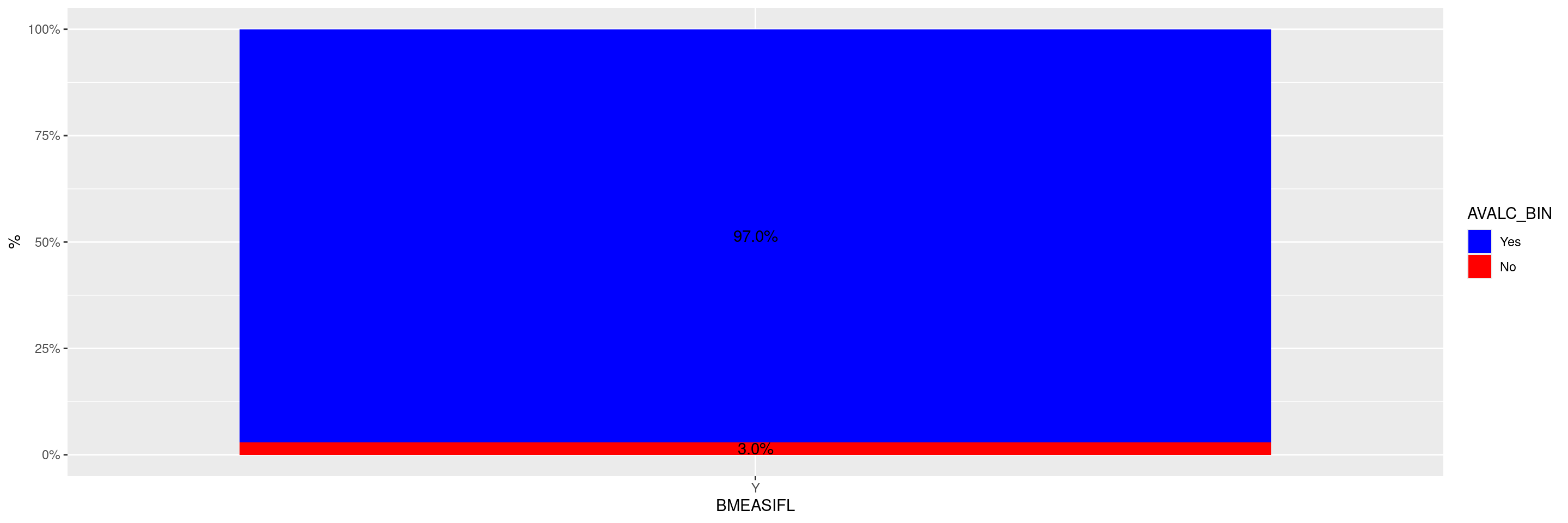
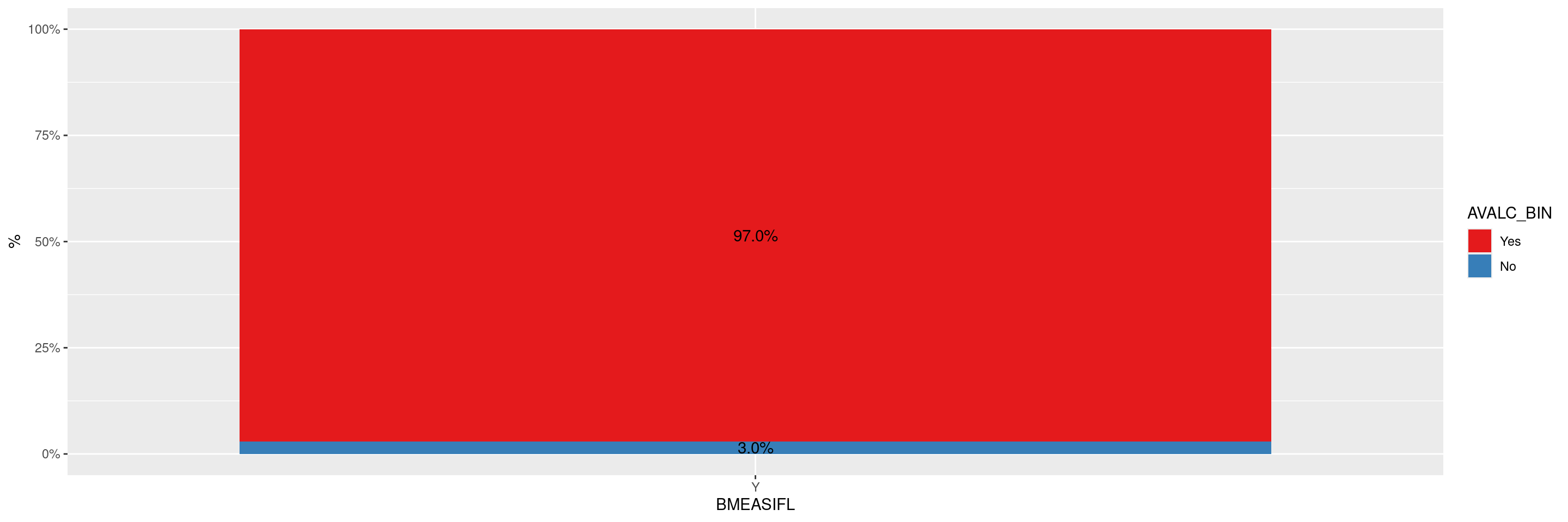
Alternatively we can also use the scale_fill_brewer() function from ggplot2 to change the color scheme of the plot by selecting a preset color palette.

Code

graph +
  scale_fill_brewer(palette = "Set1")

Code

sessionInfo()

R version 4.4.2 (2024-10-31)
Platform: x86_64-pc-linux-gnu
Running under: Ubuntu 24.04.1 LTS

Matrix products: default
BLAS:   /usr/lib/x86_64-linux-gnu/openblas-pthread/libblas.so.3 
LAPACK: /usr/lib/x86_64-linux-gnu/openblas-pthread/libopenblasp-r0.3.26.so;  LAPACK version 3.12.0

locale:
 [1] LC_CTYPE=en_US.UTF-8       LC_NUMERIC=C              
 [3] LC_TIME=en_US.UTF-8        LC_COLLATE=en_US.UTF-8    
 [5] LC_MONETARY=en_US.UTF-8    LC_MESSAGES=en_US.UTF-8   
 [7] LC_PAPER=en_US.UTF-8       LC_NAME=C                 
 [9] LC_ADDRESS=C               LC_TELEPHONE=C            
[11] LC_MEASUREMENT=en_US.UTF-8 LC_IDENTIFICATION=C       

time zone: Etc/UTC
tzcode source: system (glibc)

attached base packages:
[1] stats     graphics  grDevices utils     datasets  methods   base     

other attached packages:
[1] dplyr_1.1.4         ggplot2.utils_0.3.2 ggplot2_3.5.1      
[4] tern_0.9.7          rtables_0.6.11      magrittr_2.0.3     
[7] formatters_0.5.10  

loaded via a namespace (and not attached):
 [1] generics_0.1.3           tidyr_1.3.1              EnvStats_3.0.0          
 [4] stringi_1.8.4            lattice_0.22-6           digest_0.6.37           
 [7] RColorBrewer_1.1-3       evaluate_1.0.3           grid_4.4.2              
[10] fastmap_1.2.0            jsonlite_1.9.0           Matrix_1.7-2            
[13] backports_1.5.0          survival_3.8-3           purrr_1.0.4             
[16] scales_1.3.0             codetools_0.2-20         Rdpack_2.6.2            
[19] cli_3.6.4                ggpp_0.5.8-1             nestcolor_0.1.3         
[22] rlang_1.1.5              rbibutils_2.3            munsell_0.5.1           
[25] splines_4.4.2            withr_3.0.2              yaml_2.3.10             
[28] tools_4.4.2              polynom_1.4-1            checkmate_2.3.2         
[31] colorspace_2.1-1         forcats_1.0.0            ggstats_0.8.0           
[34] broom_1.0.7              vctrs_0.6.5              R6_2.6.1                
[37] lifecycle_1.0.4          stringr_1.5.1            htmlwidgets_1.6.4       
[40] MASS_7.3-64              pkgconfig_2.0.3          pillar_1.10.1           
[43] gtable_0.3.6             glue_1.8.0               xfun_0.51               
[46] tibble_3.2.1             tidyselect_1.2.1         knitr_1.49              
[49] farver_2.1.2             htmltools_0.5.8.1        labeling_0.4.3          
[52] rmarkdown_2.29           random.cdisc.data_0.3.16 compiler_4.4.2

Reuse