SFG3A

Comparing Between Genders in Survival Forest Graph for One Treatment Arm

SFG

We prepare the data similarly as in SFG1, focusing on a single arm in the biomarker evaluable population.

Code

library(tern)
library(dplyr)

adtte <- random.cdisc.data::cadtte %>%
  df_explicit_na() %>%
  filter(
    PARAMCD == "OS",
    ARM == "A: Drug X",
    BEP01FL == "Y"
  ) %>%
  mutate(
    AVAL = day2month(AVAL),
    AVALU = "Months",
    is_event = CNSR == 0
  ) %>%
  var_relabel(
    BEP01FL = "BEP",
    BMRKR1 = "Biomarker (Countinuous)"
  )

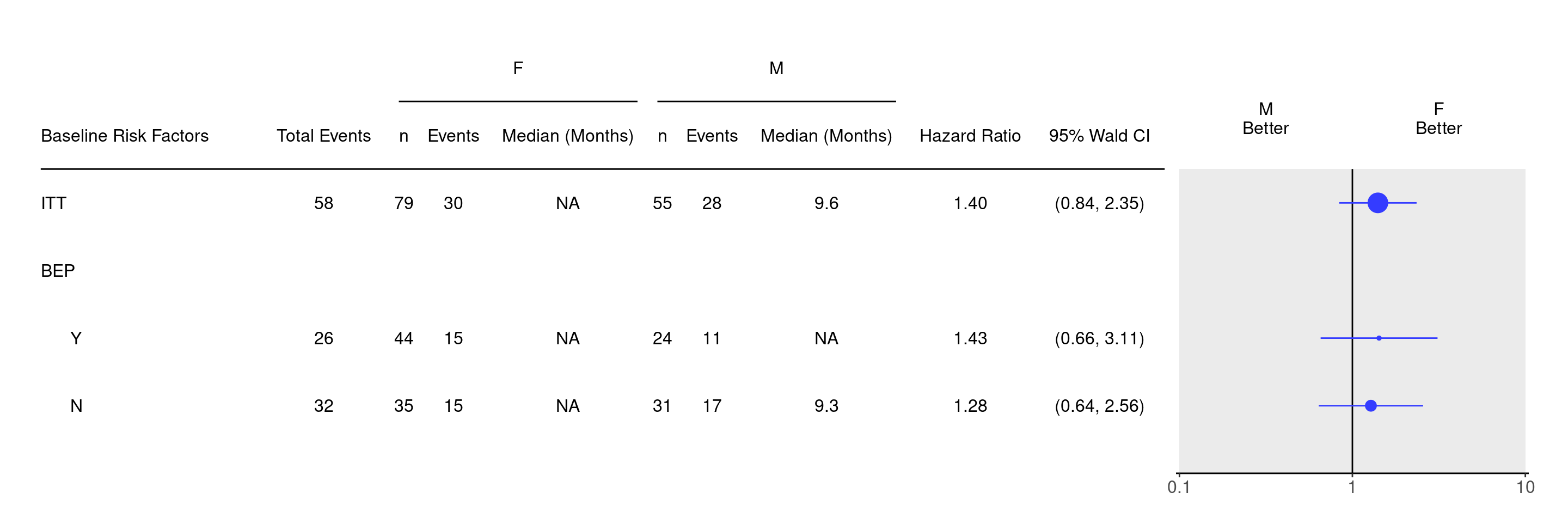
We prepare the data similarly as in SFG3. Additionally we are filtering random.cdisc.data::cadtte to keep only two categories for the SEX variable (otherwise we would not be able to do the forest plot), and we are keeping all ITT patients. We then tabulate statistics to be able to use them as an input for the forest plot.

Code

adtte_mf <- random.cdisc.data::cadtte %>%
  df_explicit_na() %>%
  filter(
    PARAMCD == "OS",
    ARM == "A: Drug X",
    SEX %in% c("M", "F")
  ) %>%
  droplevels() %>%
  mutate(
    AVAL = day2month(AVAL),
    AVALU = "Months",
    is_event = CNSR == 0
  ) %>%
  var_relabel(
    BEP01FL = "BEP",
    BMRKR1 = "Biomarker (Countinuous)"
  )

tbl <- extract_survival_subgroups(
  variables = list(
    tte = "AVAL",
    is_event = "is_event",
    arm = "SEX",
    subgroups = "BEP01FL"
  ),
  label_all = "ITT",
  data = adtte_mf
)

result <- basic_table() %>%
  tabulate_survival_subgroups(
    df = tbl,
    vars = c("n_tot_events", "n", "n_events", "median", "hr", "ci"),
    time_unit = adtte_mf$AVALU[1]
  )

We can now produce the forest plot using the g_forest() function.

Code

g_forest(result)

Code

sessionInfo()

R version 4.4.2 (2024-10-31)
Platform: x86_64-pc-linux-gnu
Running under: Ubuntu 24.04.1 LTS

Matrix products: default
BLAS:   /usr/lib/x86_64-linux-gnu/openblas-pthread/libblas.so.3 
LAPACK: /usr/lib/x86_64-linux-gnu/openblas-pthread/libopenblasp-r0.3.26.so;  LAPACK version 3.12.0

locale:
 [1] LC_CTYPE=en_US.UTF-8       LC_NUMERIC=C              
 [3] LC_TIME=en_US.UTF-8        LC_COLLATE=en_US.UTF-8    
 [5] LC_MONETARY=en_US.UTF-8    LC_MESSAGES=en_US.UTF-8   
 [7] LC_PAPER=en_US.UTF-8       LC_NAME=C                 
 [9] LC_ADDRESS=C               LC_TELEPHONE=C            
[11] LC_MEASUREMENT=en_US.UTF-8 LC_IDENTIFICATION=C       

time zone: Etc/UTC
tzcode source: system (glibc)

attached base packages:
[1] stats     graphics  grDevices utils     datasets  methods   base     

other attached packages:
[1] dplyr_1.1.4       tern_0.9.7        rtables_0.6.11    magrittr_2.0.3   
[5] formatters_0.5.10

loaded via a namespace (and not attached):
 [1] Matrix_1.7-2             gtable_0.3.6             jsonlite_1.9.0          
 [4] compiler_4.4.2           tidyselect_1.2.1         stringr_1.5.1           
 [7] tidyr_1.3.1              splines_4.4.2            scales_1.3.0            
[10] yaml_2.3.10              fastmap_1.2.0            lattice_0.22-6          
[13] ggplot2_3.5.1            R6_2.6.1                 labeling_0.4.3          
[16] generics_0.1.3           knitr_1.49               forcats_1.0.0           
[19] rbibutils_2.3            htmlwidgets_1.6.4        backports_1.5.0         
[22] checkmate_2.3.2          tibble_3.2.1             munsell_0.5.1           
[25] pillar_1.10.1            rlang_1.1.5              broom_1.0.7             
[28] stringi_1.8.4            xfun_0.51                cli_3.6.4               
[31] withr_3.0.2              Rdpack_2.6.2             digest_0.6.37           
[34] grid_4.4.2               cowplot_1.1.3            lifecycle_1.0.4         
[37] vctrs_0.6.5              evaluate_1.0.3           glue_1.8.0              
[40] farver_2.1.2             nestcolor_0.1.3          codetools_0.2-20        
[43] survival_3.8-3           random.cdisc.data_0.3.16 colorspace_2.1-1        
[46] rmarkdown_2.29           purrr_1.0.4              tools_4.4.2             
[49] pkgconfig_2.0.3          htmltools_0.5.8.1

Reuse