Biomarker Analysis Catalog - Stable
  • Stable
    • Dev
  1. Graphs
  2. SFG
  3. SFG5
  4. SFG5B
  • Index

  • Tables
    • CPMT
      • CPMT1
      • CPMT2
        • CPMT2A
      • CPMT3
    • DT
      • DT1
        • DT1A
        • DT1B
        • DT1C
      • DT2
        • DT2A
    • TET
      • TET1
        • TET1A

  • Graphs
    • AG
      • AG1
    • DG
      • DG1
        • DG1A
        • DG1B
      • DG2
      • DG3
        • DG3A
      • DG4
    • KG
      • KG1
        • KG1A
        • KG1B
      • KG2
        • KG2A
      • KG3
      • KG4
        • KG4A
        • KG4B
      • KG5
        • KG5A
        • KG5B
    • RFG
      • RFG1
        • RFG1A
      • RFG2
        • RFG2A
        • RFG2B
        • RFG2C
      • RFG3
    • RG
      • RG1
        • RG1A
        • RG1B
        • RG1C
      • RG2
        • RG2A
      • RG3
        • RG3A
        • RG3B
    • SPG
      • SPG1
      • SPG2
    • RNAG
      • RNAG1
      • RNAG2
      • RNAG3
      • RNAG4
      • RNAG5
      • RNAG6
      • RNAG7
      • RNAG8
      • RNAG9
      • RNAG10
    • SFG
      • SFG1
        • SFG1A
        • SFG1B
      • SFG2
        • SFG2A
        • SFG2B
        • SFG2C
        • SFG2D
      • SFG3
        • SFG3A
      • SFG4
      • SFG5
        • SFG5A
        • SFG5B
        • SFG5C
      • SFG6
        • SFG6A
        • SFG6B
        • SFG6C
  1. Graphs
  2. SFG
  3. SFG5
  4. SFG5B

SFG5B

Survival Forest Graph Comparing Categorical Biomarker Groups on Subgroups, including ITT

SFG

  • Setup
  • Plot
  • Session Info

We prepare the data similarly as in SFG1.

Code
library(tern)
library(dplyr)

AGE_probs <- 0.5

adtte <- random.cdisc.data::cadtte %>%
  df_explicit_na() %>%
  filter(
    PARAMCD == "OS"
  ) %>%
  mutate(
    AVAL = day2month(AVAL),
    AVALU = "Months",
    is_event = CNSR == 0,
    ARM_BIN = fct_collapse_only(
      ARM,
      CTRL = "B: Placebo",
      TRT = c("A: Drug X", "C: Combination")
    ),
    AGE_BIN = cut_quantile_bins(AGE, probs = AGE_probs),
    BMRKR2 = fct_explicit_na_if(BMRKR2, BEP01FL == "N"),
    BMRKR2_BIN = fct_collapse_only(
      BMRKR2,
      High = "HIGH",
      Low = c("MEDIUM", "LOW")
    )
  ) %>%
  var_relabel(
    BEP01FL = "BEP",
    BMRKR2_BIN = "Biomarker (Binary)"
  )

We use the same tables_all() function above and combine all subtables using rbind() to tabulate statistics to be able to use as an input for forest plot.

Code
tables_all <- function(filter_var, filter_condition, sub_var) {
  dataset <- adtte %>%
    filter(!!as.name(filter_var) == filter_condition)
  if (nrow(dataset) == 0) {
    stop(paste("Subset", filter_var, "==", filter_condition, "is empty"))
  }
  tbl <- extract_survival_subgroups(
    variables = list(
      tte = "AVAL",
      is_event = "is_event",
      arm = "ARM_BIN",
      subgroups = sub_var
    ),
    label_all = "ITT",
    data = dataset
  )
  basic_table() %>%
    tabulate_survival_subgroups(
      df = tbl,
      vars = c("n_tot_events", "n", "n_events", "median", "hr", "ci"),
      time_unit = dataset$AVALU[1]
    )
}

add_subtitle <- function(sub_tab, sub_title) {
  label_at_path(sub_tab, path = row_paths(sub_tab)[[1]][1]) <- sub_title
  sub_tab
}

tables_list <- list(
  tables_all(filter_var = "SEX", filter_condition = "F", sub_var = c("BEP01FL", "BMRKR2_BIN")),
  tables_all(filter_var = "SEX", filter_condition = "M", sub_var = c("BEP01FL", "BMRKR2_BIN")),
  tables_all(filter_var = "AGE_BIN", filter_condition = "[0%,50%]", sub_var = c("BEP01FL", "BMRKR2_BIN")),
  tables_all(filter_var = "AGE_BIN", filter_condition = "(50%,100%]", sub_var = c("BEP01FL", "BMRKR2_BIN"))
)

We can now produce the forest plot using the g_forest() function.

Code
one_table <- tables_list[[1]]
result <- rbind(
  add_subtitle(tables_list[[1]], "SEX = F"),
  add_subtitle(tables_list[[2]], "SEX = M"),
  add_subtitle(tables_list[[3]], "AGE_BIN = [0%,50%]"),
  add_subtitle(tables_list[[4]], "AGE_BIN = (50%,100%]")
)
g_forest(
  result,
  col_x = attr(one_table, "col_x"),
  col_ci = attr(one_table, "col_ci"),
  forest_header = attr(one_table, "forest_header"),
  col_symbol_size = attr(one_table, "col_symbol_size")
)

Code
sessionInfo()
R version 4.4.2 (2024-10-31)
Platform: x86_64-pc-linux-gnu
Running under: Ubuntu 24.04.1 LTS

Matrix products: default
BLAS:   /usr/lib/x86_64-linux-gnu/openblas-pthread/libblas.so.3 
LAPACK: /usr/lib/x86_64-linux-gnu/openblas-pthread/libopenblasp-r0.3.26.so;  LAPACK version 3.12.0

locale:
 [1] LC_CTYPE=en_US.UTF-8       LC_NUMERIC=C              
 [3] LC_TIME=en_US.UTF-8        LC_COLLATE=en_US.UTF-8    
 [5] LC_MONETARY=en_US.UTF-8    LC_MESSAGES=en_US.UTF-8   
 [7] LC_PAPER=en_US.UTF-8       LC_NAME=C                 
 [9] LC_ADDRESS=C               LC_TELEPHONE=C            
[11] LC_MEASUREMENT=en_US.UTF-8 LC_IDENTIFICATION=C       

time zone: Etc/UTC
tzcode source: system (glibc)

attached base packages:
[1] stats     graphics  grDevices utils     datasets  methods   base     

other attached packages:
[1] dplyr_1.1.4       tern_0.9.7        rtables_0.6.11    magrittr_2.0.3   
[5] formatters_0.5.10

loaded via a namespace (and not attached):
 [1] Matrix_1.7-2             gtable_0.3.6             jsonlite_1.9.0          
 [4] compiler_4.4.2           tidyselect_1.2.1         stringr_1.5.1           
 [7] tidyr_1.3.1              splines_4.4.2            scales_1.3.0            
[10] yaml_2.3.10              fastmap_1.2.0            lattice_0.22-6          
[13] ggplot2_3.5.1            R6_2.6.1                 labeling_0.4.3          
[16] generics_0.1.3           knitr_1.49               forcats_1.0.0           
[19] rbibutils_2.3            htmlwidgets_1.6.4        backports_1.5.0         
[22] checkmate_2.3.2          tibble_3.2.1             munsell_0.5.1           
[25] pillar_1.10.1            rlang_1.1.5              broom_1.0.7             
[28] stringi_1.8.4            xfun_0.51                cli_3.6.4               
[31] withr_3.0.2              Rdpack_2.6.2             digest_0.6.37           
[34] grid_4.4.2               cowplot_1.1.3            lifecycle_1.0.4         
[37] vctrs_0.6.5              evaluate_1.0.3           glue_1.8.0              
[40] farver_2.1.2             nestcolor_0.1.3          codetools_0.2-20        
[43] survival_3.8-3           random.cdisc.data_0.3.16 colorspace_2.1-1        
[46] rmarkdown_2.29           purrr_1.0.4              tools_4.4.2             
[49] pkgconfig_2.0.3          htmltools_0.5.8.1       

Reuse

Copyright 2023, Hoffmann-La Roche Ltd.
SFG5A
SFG5C
Source Code
---
title: SFG5B
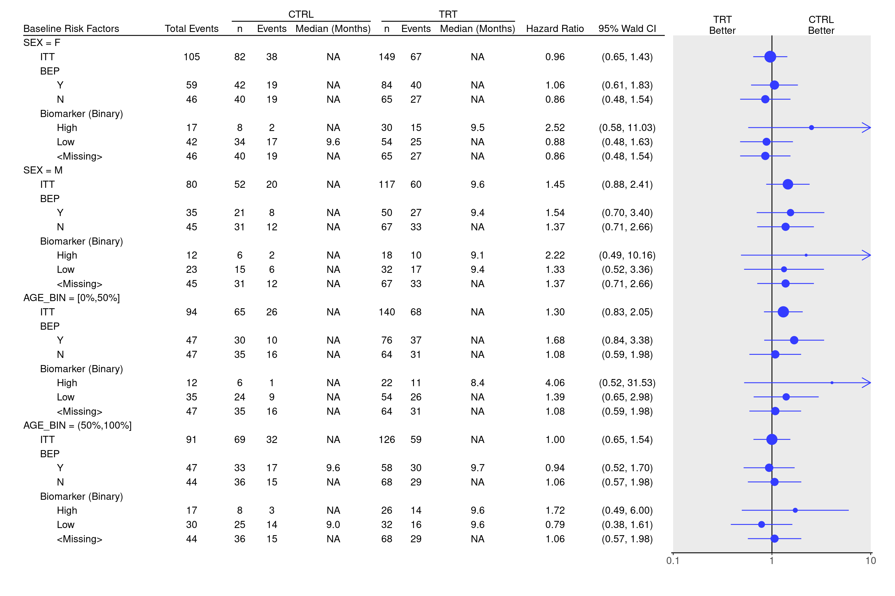
subtitle: Survival Forest Graph Comparing Categorical Biomarker Groups on Subgroups, including ITT
categories: [SFG]
---

------------------------------------------------------------------------

::: panel-tabset
{{< include setup.qmd >}}

## Plot

We use the same `tables_all()` function above and combine all subtables using `rbind()` to tabulate statistics to be able to use as an input for forest plot.

```{r}
tables_all <- function(filter_var, filter_condition, sub_var) {
  dataset <- adtte %>%
    filter(!!as.name(filter_var) == filter_condition)
  if (nrow(dataset) == 0) {
    stop(paste("Subset", filter_var, "==", filter_condition, "is empty"))
  }
  tbl <- extract_survival_subgroups(
    variables = list(
      tte = "AVAL",
      is_event = "is_event",
      arm = "ARM_BIN",
      subgroups = sub_var
    ),
    label_all = "ITT",
    data = dataset
  )
  basic_table() %>%
    tabulate_survival_subgroups(
      df = tbl,
      vars = c("n_tot_events", "n", "n_events", "median", "hr", "ci"),
      time_unit = dataset$AVALU[1]
    )
}

add_subtitle <- function(sub_tab, sub_title) {
  label_at_path(sub_tab, path = row_paths(sub_tab)[[1]][1]) <- sub_title
  sub_tab
}

tables_list <- list(
  tables_all(filter_var = "SEX", filter_condition = "F", sub_var = c("BEP01FL", "BMRKR2_BIN")),
  tables_all(filter_var = "SEX", filter_condition = "M", sub_var = c("BEP01FL", "BMRKR2_BIN")),
  tables_all(filter_var = "AGE_BIN", filter_condition = "[0%,50%]", sub_var = c("BEP01FL", "BMRKR2_BIN")),
  tables_all(filter_var = "AGE_BIN", filter_condition = "(50%,100%]", sub_var = c("BEP01FL", "BMRKR2_BIN"))
)
```

We can now produce the forest plot using the `g_forest()` function.

```{r, fig.width = 15, fig.height = 10}
one_table <- tables_list[[1]]
result <- rbind(
  add_subtitle(tables_list[[1]], "SEX = F"),
  add_subtitle(tables_list[[2]], "SEX = M"),
  add_subtitle(tables_list[[3]], "AGE_BIN = [0%,50%]"),
  add_subtitle(tables_list[[4]], "AGE_BIN = (50%,100%]")
)
g_forest(
  result,
  col_x = attr(one_table, "col_x"),
  col_ci = attr(one_table, "col_ci"),
  forest_header = attr(one_table, "forest_header"),
  col_symbol_size = attr(one_table, "col_symbol_size")
)
```

{{< include ../../misc/session_info.qmd >}}
:::

Made with ❤️ by the Statistical Engineering Team StatisticalEngineering

  • License

  • Edit this page
  • Report an issue
Cookie Preferences