SFG1B

Survival Forest Graph Only by Binned Continuous Variable

SFG

We will use the cadtte data set from the random.cdisc.data package to create the survival forest graph. We start by filtering the adtte data set for the overall survival observations, converting time of overall survival to months, creating a new variable for event information, binarizing the ARM variable and creating a binned age variable by using the function cut_quantile_bins(). Note that we do not include the boundaries 0 and 1 in the corresponding cutoffs vector AGE_probs, but only the true cutoff probabilities to use (here 0.5, i.e. the median). We restrict the analysis of the biomarker variables BMRKR1 and BMRKR2 to the BEP by setting them as missing for the non-BEP.

We also relabel the biomarker evaluable population flag variable BEP01FL and the categorical biomarker variable BMRKR2 to update the display label of these variables in the graph.

Code

library(tern)
library(dplyr)

AGE_probs <- 0.5

adtte <- random.cdisc.data::cadtte %>%
  df_explicit_na() %>%
  filter(
    PARAMCD == "OS"
  ) %>%
  mutate(
    AVAL = day2month(AVAL),
    AVALU = "Months",
    is_event = CNSR == 0,
    ARM_BIN = fct_collapse_only(
      ARM,
      CTRL = "B: Placebo",
      TRT = c("A: Drug X", "C: Combination")
    ),
    AGE_BIN = cut_quantile_bins(AGE, probs = AGE_probs),
    BMRKR1 = ifelse(BEP01FL == "N", NA, BMRKR1),
    BMRKR2 = fct_explicit_na_if(BMRKR2, BEP01FL == "N")
  ) %>%
  var_relabel(
    BEP01FL = "BEP",
    BMRKR2 = "Biomarker (Categorical)"
  )

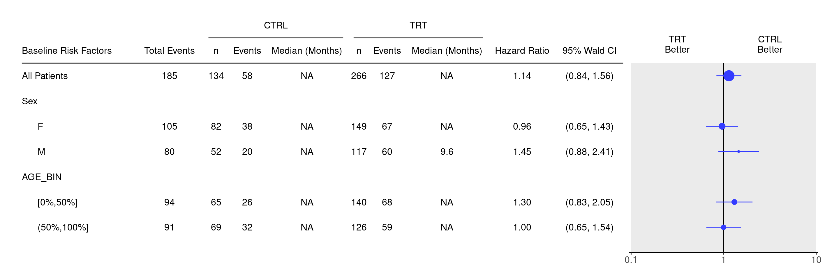
This works analogously to SFG1, we just specify different factor variables in subgroups, here including the binned continuous variable AGE_BIN as well as SEX.

Code

tbl <- extract_survival_subgroups(
  variables = list(
    tte = "AVAL",
    is_event = "is_event",
    arm = "ARM_BIN",
    subgroups = c("SEX", "AGE_BIN")
  ),
  data = adtte
)

result <- basic_table() %>%
  tabulate_survival_subgroups(
    df = tbl,
    vars = c("n_tot_events", "n", "n_events", "median", "hr", "ci"),
    time_unit = adtte$AVALU[1]
  )

We can now produce the forest plot using g_forest().

Code

g_forest(result)

Code

sessionInfo()

R version 4.4.2 (2024-10-31)
Platform: x86_64-pc-linux-gnu
Running under: Ubuntu 24.04.1 LTS

Matrix products: default
BLAS:   /usr/lib/x86_64-linux-gnu/openblas-pthread/libblas.so.3 
LAPACK: /usr/lib/x86_64-linux-gnu/openblas-pthread/libopenblasp-r0.3.26.so;  LAPACK version 3.12.0

locale:
 [1] LC_CTYPE=en_US.UTF-8       LC_NUMERIC=C              
 [3] LC_TIME=en_US.UTF-8        LC_COLLATE=en_US.UTF-8    
 [5] LC_MONETARY=en_US.UTF-8    LC_MESSAGES=en_US.UTF-8   
 [7] LC_PAPER=en_US.UTF-8       LC_NAME=C                 
 [9] LC_ADDRESS=C               LC_TELEPHONE=C            
[11] LC_MEASUREMENT=en_US.UTF-8 LC_IDENTIFICATION=C       

time zone: Etc/UTC
tzcode source: system (glibc)

attached base packages:
[1] stats     graphics  grDevices utils     datasets  methods   base     

other attached packages:
[1] dplyr_1.1.4       tern_0.9.7        rtables_0.6.11    magrittr_2.0.3   
[5] formatters_0.5.10

loaded via a namespace (and not attached):
 [1] Matrix_1.7-2             gtable_0.3.6             jsonlite_1.9.0          
 [4] compiler_4.4.2           tidyselect_1.2.1         stringr_1.5.1           
 [7] tidyr_1.3.1              splines_4.4.2            scales_1.3.0            
[10] yaml_2.3.10              fastmap_1.2.0            lattice_0.22-6          
[13] ggplot2_3.5.1            R6_2.6.1                 labeling_0.4.3          
[16] generics_0.1.3           knitr_1.49               forcats_1.0.0           
[19] rbibutils_2.3            htmlwidgets_1.6.4        backports_1.5.0         
[22] checkmate_2.3.2          tibble_3.2.1             munsell_0.5.1           
[25] pillar_1.10.1            rlang_1.1.5              broom_1.0.7             
[28] stringi_1.8.4            xfun_0.51                cli_3.6.4               
[31] withr_3.0.2              Rdpack_2.6.2             digest_0.6.37           
[34] grid_4.4.2               cowplot_1.1.3            lifecycle_1.0.4         
[37] vctrs_0.6.5              evaluate_1.0.3           glue_1.8.0              
[40] farver_2.1.2             nestcolor_0.1.3          codetools_0.2-20        
[43] survival_3.8-3           random.cdisc.data_0.3.16 colorspace_2.1-1        
[46] rmarkdown_2.29           purrr_1.0.4              tools_4.4.2             
[49] pkgconfig_2.0.3          htmltools_0.5.8.1

Reuse