RFG1A

Response Forest Graph Only by Categorical or Binned Continuous Biomarker

RFG

These templates are helpful when we are interested in the odds ratios between two groups, usually two treatment arms. We would like to assess how the odds ratio changes when we look at different subgroups, often defined by categorical biomarker variables, e.g.

We will use the cadrs data set from the random.cdisc.data package to create the response forest graph. We start by filtering the adrs data set for the Best Confirmed Overall Response by Investigator and patients with measurable disease at baseline (BMEASIFL == "Y"). We create a new variable for response information (we define response patients to include CR and PR patients), and binarize the ARM variable. We also fix a data artifact by setting the categorical biomarker variable BMRKR2 to an explicit <Missing> level for the non-biomarker evaluable population.

We also relabel the biomarker evaluable population flag variable BEP01FL and the categorical biomarker variable BMRKR2 to update the display label of these variables in the graph.

Code

library(tern)
library(ggplot2.utils)
library(dplyr)

adrs <- random.cdisc.data::cadrs %>%
  df_explicit_na() %>%
  filter(PARAMCD == "BESRSPI", BMEASIFL == "Y") %>%
  mutate(
    is_rsp = AVALC %in% c("CR", "PR"),
    ARM_BIN = fct_collapse_only(
      ARM,
      CTRL = c("B: Placebo"),
      TRT = c("A: Drug X", "C: Combination")
    ),
    BMRKR2 = fct_explicit_na_if(BMRKR2, BEP01FL == "N")
  ) %>%
  var_relabel(
    BEP01FL = "BEP",
    BMRKR2 = "Biomarker (Categorical)"
  )

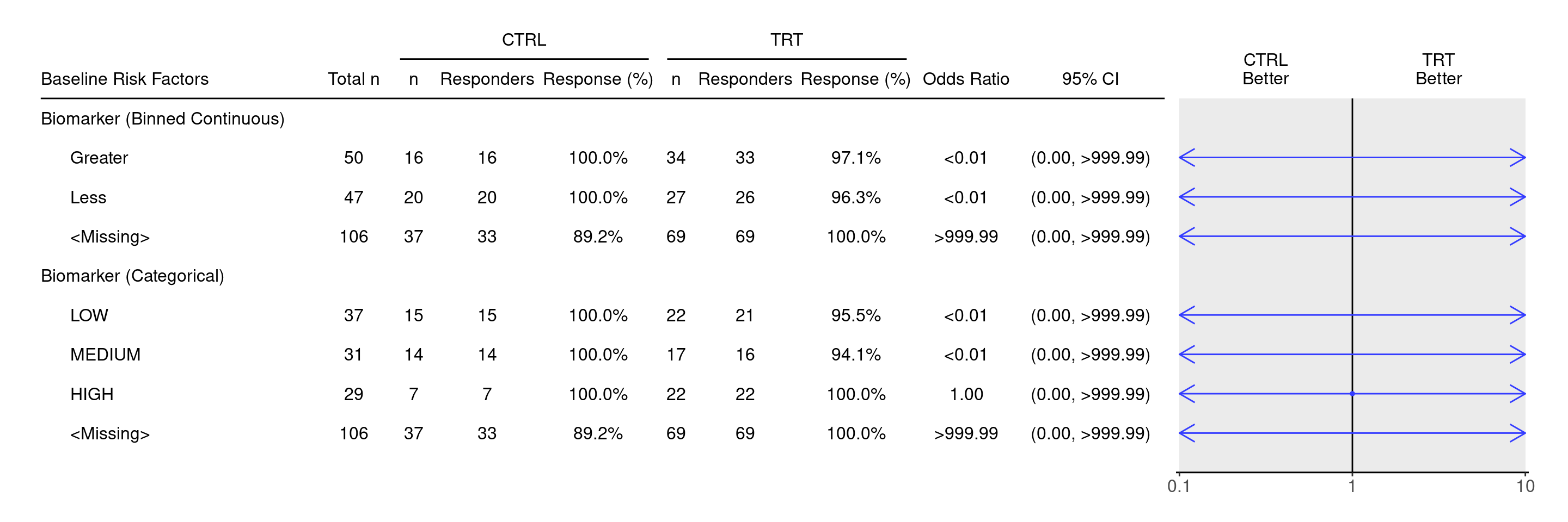
We define a binned factor variable BMRKR1_cut from the continuous biomarker variable BMRKR1 to illustrate. Note that the remaining code would work the same for an originally categorical biomarker.

Code

BMRKR1_cutpoint <- 5

adrs2 <- adrs %>%
  mutate(
    BMRKR1 = ifelse(BEP01FL == "N", NA, BMRKR1),
    BMRKR1_cut = explicit_na(factor(
      ifelse(BMRKR1 > BMRKR1_cutpoint, "Greater", "Less")
    ))
  ) %>%
  var_relabel(BMRKR1_cut = "Biomarker (Binned Continuous)")

df <- extract_rsp_subgroups(
  variables = list(
    rsp = "is_rsp",
    arm = "ARM_BIN",
    subgroups = c("BMRKR1_cut", "BMRKR2")
  ),
  data = adrs2,
  conf_level = 0.95
)

result <- basic_table() %>%
  tabulate_rsp_subgroups(df, vars = c("n_tot", "n", "n_rsp", "prop", "or", "ci"))

We can remove the first line showing the All Patients category from the result table as follows.

Code

result <- result[-1, , keep_topleft = TRUE]

We can then produce the forest plot again using g_forest() on this trimmed result table.

Code

g_forest(result)

Code

sessionInfo()

R version 4.4.2 (2024-10-31)
Platform: x86_64-pc-linux-gnu
Running under: Ubuntu 24.04.1 LTS

Matrix products: default
BLAS:   /usr/lib/x86_64-linux-gnu/openblas-pthread/libblas.so.3 
LAPACK: /usr/lib/x86_64-linux-gnu/openblas-pthread/libopenblasp-r0.3.26.so;  LAPACK version 3.12.0

locale:
 [1] LC_CTYPE=en_US.UTF-8       LC_NUMERIC=C              
 [3] LC_TIME=en_US.UTF-8        LC_COLLATE=en_US.UTF-8    
 [5] LC_MONETARY=en_US.UTF-8    LC_MESSAGES=en_US.UTF-8   
 [7] LC_PAPER=en_US.UTF-8       LC_NAME=C                 
 [9] LC_ADDRESS=C               LC_TELEPHONE=C            
[11] LC_MEASUREMENT=en_US.UTF-8 LC_IDENTIFICATION=C       

time zone: Etc/UTC
tzcode source: system (glibc)

attached base packages:
[1] stats     graphics  grDevices utils     datasets  methods   base     

other attached packages:
[1] dplyr_1.1.4         ggplot2.utils_0.3.2 ggplot2_3.5.1      
[4] tern_0.9.7          rtables_0.6.11      magrittr_2.0.3     
[7] formatters_0.5.10  

loaded via a namespace (and not attached):
 [1] generics_0.1.3           tidyr_1.3.1              EnvStats_3.0.0          
 [4] stringi_1.8.4            lattice_0.22-6           digest_0.6.37           
 [7] evaluate_1.0.3           grid_4.4.2               fastmap_1.2.0           
[10] jsonlite_1.9.0           Matrix_1.7-2             backports_1.5.0         
[13] survival_3.8-3           purrr_1.0.4              scales_1.3.0            
[16] codetools_0.2-20         Rdpack_2.6.2             cli_3.6.4               
[19] ggpp_0.5.8-1             nestcolor_0.1.3          rlang_1.1.5             
[22] rbibutils_2.3            cowplot_1.1.3            munsell_0.5.1           
[25] splines_4.4.2            withr_3.0.2              yaml_2.3.10             
[28] tools_4.4.2              polynom_1.4-1            checkmate_2.3.2         
[31] colorspace_2.1-1         forcats_1.0.0            ggstats_0.8.0           
[34] broom_1.0.7              vctrs_0.6.5              R6_2.6.1                
[37] lifecycle_1.0.4          stringr_1.5.1            htmlwidgets_1.6.4       
[40] MASS_7.3-64              pkgconfig_2.0.3          pillar_1.10.1           
[43] gtable_0.3.6             glue_1.8.0               xfun_0.51               
[46] tibble_3.2.1             tidyselect_1.2.1         knitr_1.49              
[49] farver_2.1.2             htmltools_0.5.8.1        labeling_0.4.3          
[52] rmarkdown_2.29           random.cdisc.data_0.3.16 compiler_4.4.2

Reuse