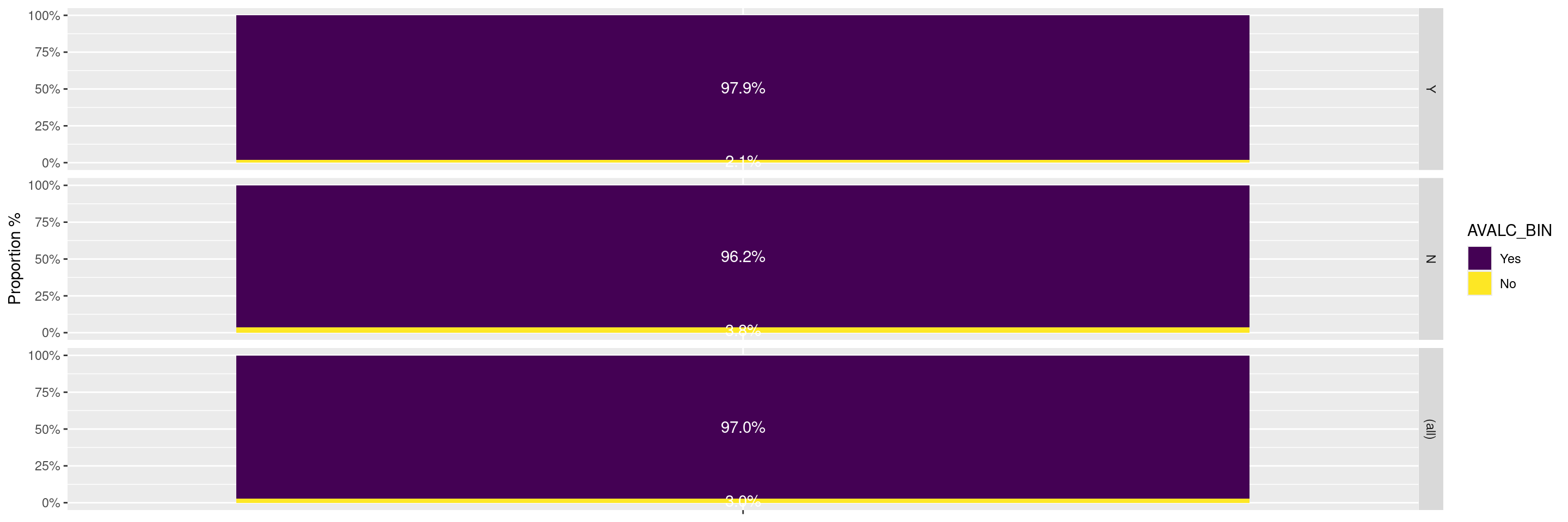
In this example we can use the facet_grid() layer with the margins = TRUE option to compare the responses between the biomarker evaluable population (BEP) and the overall population.
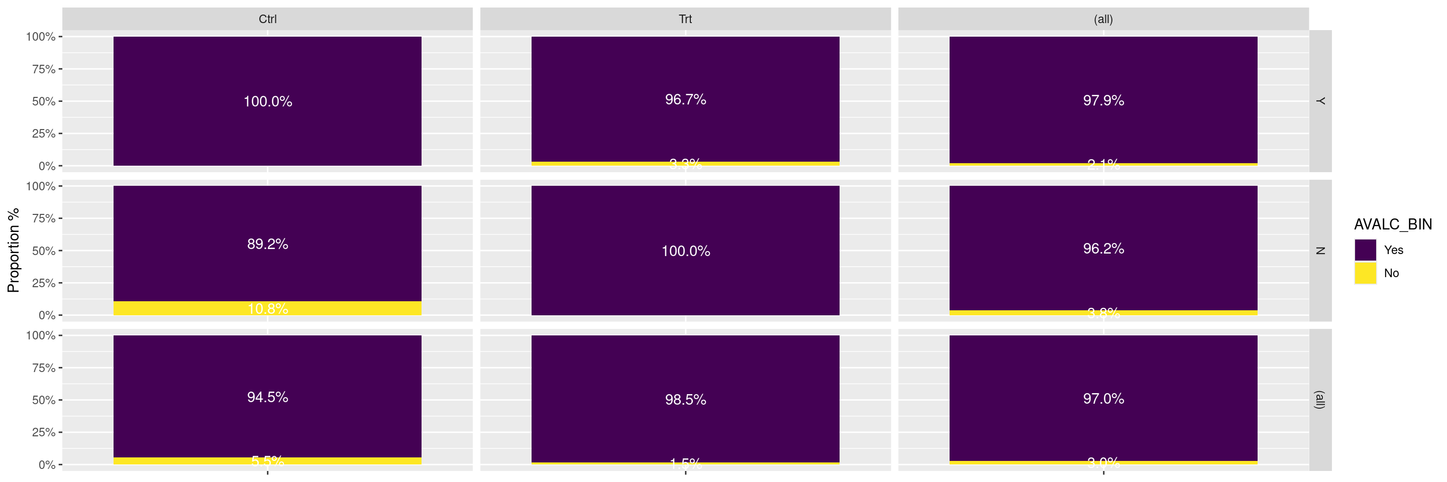
In this example we compare the responses across treatment arms between the biomarker evaluable population and the full population. We can add the option margins = TRUE option within the facet_grid() layer to obtain the responses across all treatment arms and their combination within each of the populations.
---title: RG3subtitle: Response Graphs Comparing BEP vs. Overall Populationcategories: [RG]---------------------------------------------------------------------------::: panel-tabset{{< include setup.qmd >}}## PlotIn this example we can use the `facet_grid()` layer with the `margins = TRUE` option to compare the responses between the biomarker evaluable population (BEP) and the overall population.```{r}graph <-ggplot(adrs, aes(BMEASIFL, fill = AVALC_BIN, by = BMEASIFL)) +geom_bar(position ="fill") +geom_text(stat ="prop", position =position_fill(.5), colour ="white") +scale_y_continuous(labels = scales::percent,name ="Proportion %" ) +scale_x_discrete(labels =NULL) +xlab(NULL)graph +facet_grid(BEP01FL ~ ., margins =TRUE)```In this example we compare the responses across treatment arms between the biomarker evaluable population and the full population.We can add the option `margins = TRUE` option within the `facet_grid()` layer to obtain the responses across all treatment arms and their combination within each of the populations.```{r}graph +facet_grid(BEP01FL ~ ARM_BIN, margins =TRUE)```{{< include ../../misc/session_info.qmd >}}:::