RNAG10

RNAseq Survival Forest Graph

RNAG

This page can be used as a template of how to produce survival forest graphs for RNA-seq gene expression analysis using available tern and hermes functions, and to create an interactive survival forest graph for RNA-seq gene expression analysis using teal.modules.hermes.

The code below needs both RNA-seq data (in HermesData format) and time-to-event data (in ADTTE format) as input.

We first prepare the time-to-event data. We define an event indicator variable, transform the time to months and filter down to the overall survival subset.

Code

library(tern)

adtte_f <- random.cdisc.data::cadtte %>%
  dplyr::mutate(
    is_event = .data$CNSR == 0,
    AVAL = day2month(.data$AVAL),
    AVALU = "Months"
  ) %>%
  dplyr::filter(.data$PARAMCD == "OS")

Then we prepare the RNA-seq data and join with ADTTE, see RNAG9 for details.

Code

library(hermes)

gene_data <- col_data_with_genes(
  object = hermes_data,
  assay_name = "counts",
  genes = gene_spec("GeneID:1820")
)
joined_data <- inner_join_cdisc(
  gene_data = gene_data,
  cdisc_data = adtte_f
)

We can then cut the resulting gene column in the joined adtte_data into quantile bins. In this example we want two equally sized groups so set probs to 0.5, and we then label the bins as Low and High. We could choose a different quantile cutoff. The only important restriction here is that we need to bin the genes into exactly two groups, otherwise the forest plot below cannot compare these two groups with each other.

Code

arm_name <- attr(gene_data, "gene_cols")
binned_data <- joined_data %>%
  dplyr::mutate(
    gene_factor = cut_quantile_bins(
      joined_data[[arm_name]],
      probs = 0.5,
      labels = c("Low", "High")
    )
  ) %>%
  df_explicit_na(omit_columns = "AVALU")

It is now simple to create the survival forest graph by providing the data set created above with the variable specification. First we calculate the survival estimates with extract_survival_subgroups() by providing the necessary variable specification. Here we specify our derived gene_bin for the arm. Then we build the table portion with tabulate_survival_subgroups() and pass our calculations from the previous step. Lastly, we generate the final graph with g_forest.

Code

variables <- list(
  tte = "AVAL",
  is_event = "is_event",
  arm = "gene_factor",
  subgroups = c("BEP01FL", "SAFFL")
)
tbl <- extract_survival_subgroups(
  variables = variables,
  data = binned_data
)

Warning in coxph.fit(X, Y, istrat, offset, init, control, weights = weights, :
Loglik converged before variable 1 ; coefficient may be infinite.

Code

lyt <- basic_table()
result <- tabulate_survival_subgroups(
  lyt = lyt,
  df = tbl,
  vars = c("n_tot_events", "n", "n_events", "median", "hr", "ci"),
  time_unit = binned_data$AVALU[1]
)

g_forest(result)

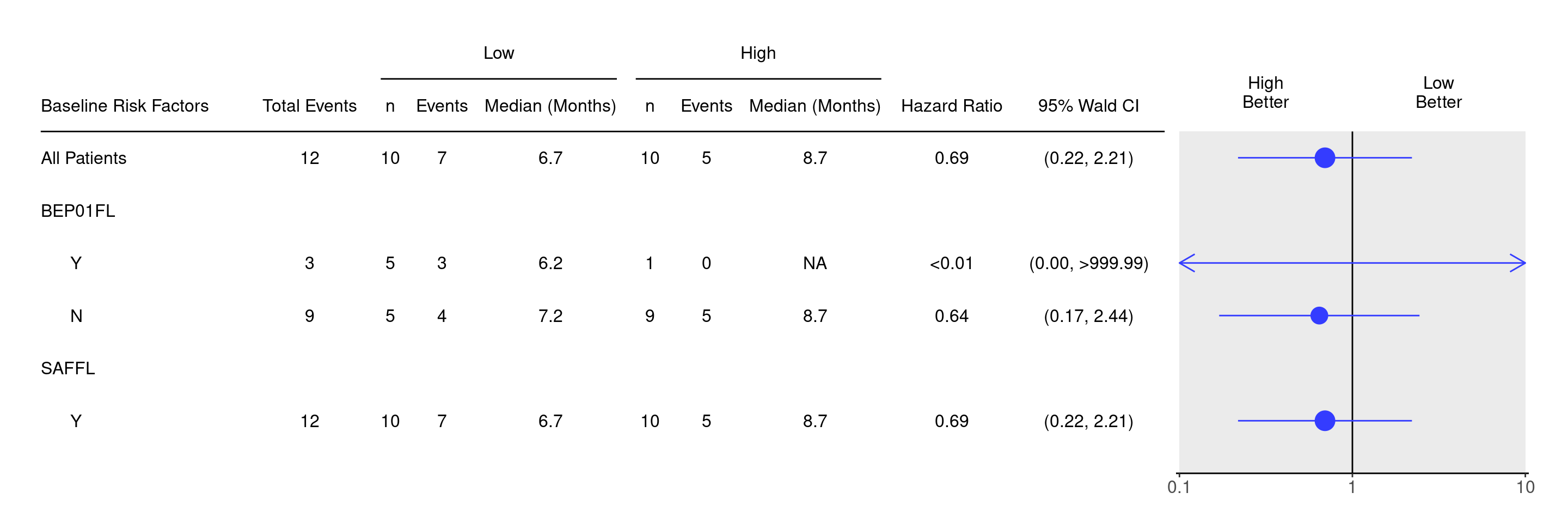
See SFG01 to SFG05 for additional customization options for the survival forest graphs or the help page ?g_forest().

We start by importing a MultiAssayExperiment and sample ADTTE data; here we use the example multi_assay_experiment available in hermes and example ADTTE data from random.cdisc.data. We can then use the provided teal module tm_g_forest_tte to include the corresponding interactive survival forest analysis in our teal app. In case that we have different non-standard column names in our ADTTE data set we could also specify them via the adtte_vars argument, see the documentation ?tm_g_forest_tte for more details.

Code

library(teal.modules.hermes)

data <- teal_data()
data <- within(data, {
  library(random.cdisc.data)
  library(dplyr)
  library(hermes)
  MAE <- multi_assay_experiment
  ADTTE <- random.cdisc.data::cadtte %>%
    mutate(is_event = .data$CNSR == 0)
})
datanames(data) <- c("MAE", "ADTTE")

Warning: `datanames<-()` was deprecated in teal.data 0.7.0.
ℹ invalid to use `datanames()<-` or `names()<-` on an object of class
  `teal_data`. See ?names.teal_data

Code

join_keys(data)["ADTTE", "ADTTE"] <- c("STUDYID", "USUBJID", "PARAMCD")

app <- init(
  data = data,
  modules = modules(
    tm_g_forest_tte(
      label = "forest",
      adtte_name = "ADTTE",
      mae_name = "MAE"
    )
  )
)

[INFO] 2025-02-19 17:34:26.1078 pid:8787 token:[] teal.modules.hermes Initializing tm_g_forest_tte

Code

shinyApp(app$ui, app$server)

Warning: 'experiments' dropped; see 'drops()'

Code

sessionInfo()

R version 4.4.2 (2024-10-31)
Platform: x86_64-pc-linux-gnu
Running under: Ubuntu 24.04.1 LTS

Matrix products: default
BLAS:   /usr/lib/x86_64-linux-gnu/openblas-pthread/libblas.so.3 
LAPACK: /usr/lib/x86_64-linux-gnu/openblas-pthread/libopenblasp-r0.3.26.so;  LAPACK version 3.12.0

locale:
 [1] LC_CTYPE=en_US.UTF-8       LC_NUMERIC=C              
 [3] LC_TIME=en_US.UTF-8        LC_COLLATE=en_US.UTF-8    
 [5] LC_MONETARY=en_US.UTF-8    LC_MESSAGES=en_US.UTF-8   
 [7] LC_PAPER=en_US.UTF-8       LC_NAME=C                 
 [9] LC_ADDRESS=C               LC_TELEPHONE=C            
[11] LC_MEASUREMENT=en_US.UTF-8 LC_IDENTIFICATION=C       

time zone: Etc/UTC
tzcode source: system (glibc)

attached base packages:
[1] stats4    stats     graphics  grDevices utils     datasets  methods  
[8] base     

other attached packages:
 [1] dplyr_1.1.4                 random.cdisc.data_0.3.16   
 [3] teal.modules.hermes_0.1.6   teal_0.16.0                
 [5] teal.slice_0.6.0            teal.data_0.7.0            
 [7] teal.code_0.6.1             shiny_1.10.0               
 [9] hermes_1.10.0               SummarizedExperiment_1.36.0
[11] Biobase_2.66.0              GenomicRanges_1.58.0       
[13] GenomeInfoDb_1.42.3         IRanges_2.40.1             
[15] S4Vectors_0.44.0            BiocGenerics_0.52.0        
[17] MatrixGenerics_1.18.1       matrixStats_1.5.0          
[19] ggfortify_0.4.17            ggplot2_3.5.1              
[21] tern_0.9.7                  rtables_0.6.11             
[23] magrittr_2.0.3              formatters_0.5.10          

loaded via a namespace (and not attached):
  [1] RColorBrewer_1.1-3          jsonlite_1.9.0             
  [3] shape_1.4.6.1               nestcolor_0.1.3            
  [5] MultiAssayExperiment_1.32.0 farver_2.1.2               
  [7] rmarkdown_2.29              GlobalOptions_0.1.2        
  [9] zlibbioc_1.52.0             vctrs_0.6.5                
 [11] memoise_2.0.1               webshot_0.5.5              
 [13] BiocBaseUtils_1.9.0         htmltools_0.5.8.1          
 [15] S4Arrays_1.6.0              forcats_1.0.0              
 [17] progress_1.2.3              curl_6.2.1                 
 [19] broom_1.0.7                 SparseArray_1.6.1          
 [21] sass_0.4.9                  bslib_0.9.0                
 [23] fontawesome_0.5.3           htmlwidgets_1.6.4          
 [25] httr2_1.1.0                 cachem_1.1.0               
 [27] teal.widgets_0.4.3          mime_0.12                  
 [29] lifecycle_1.0.4             iterators_1.0.14           
 [31] pkgconfig_2.0.3             webshot2_0.1.1             
 [33] Matrix_1.7-2                R6_2.6.1                   
 [35] fastmap_1.2.0               GenomeInfoDbData_1.2.13    
 [37] rbibutils_2.3               clue_0.3-66                
 [39] digest_0.6.37               colorspace_2.1-1           
 [41] shinycssloaders_1.1.0       ps_1.9.0                   
 [43] AnnotationDbi_1.68.0        RSQLite_2.3.9              
 [45] filelock_1.0.3              labeling_0.4.3             
 [47] httr_1.4.7                  abind_1.4-8                
 [49] compiler_4.4.2              bit64_4.6.0-1              
 [51] withr_3.0.2                 doParallel_1.0.17          
 [53] backports_1.5.0             DBI_1.2.3                  
 [55] logger_0.4.0                biomaRt_2.62.1             
 [57] rappdirs_0.3.3              DelayedArray_0.32.0        
 [59] rjson_0.2.23                chromote_0.4.0             
 [61] tools_4.4.2                 httpuv_1.6.15              
 [63] glue_1.8.0                  callr_3.7.6                
 [65] promises_1.3.2              grid_4.4.2                 
 [67] checkmate_2.3.2             cluster_2.1.8              
 [69] generics_0.1.3              gtable_0.3.6               
 [71] websocket_1.4.2             tidyr_1.3.1                
 [73] hms_1.1.3                   xml2_1.3.6                 
 [75] XVector_0.46.0              ggrepel_0.9.6              
 [77] foreach_1.5.2               pillar_1.10.1              
 [79] stringr_1.5.1               later_1.4.1                
 [81] circlize_0.4.16             splines_4.4.2              
 [83] BiocFileCache_2.14.0        lattice_0.22-6             
 [85] survival_3.8-3              bit_4.5.0.1                
 [87] tidyselect_1.2.1            ComplexHeatmap_2.22.0      
 [89] Biostrings_2.74.1           knitr_1.49                 
 [91] gridExtra_2.3               teal.logger_0.3.2          
 [93] xfun_0.51                   stringi_1.8.4              
 [95] UCSC.utils_1.2.0            yaml_2.3.10                
 [97] shinyWidgets_0.8.7          evaluate_1.0.3             
 [99] codetools_0.2-20            tibble_3.2.1               
[101] cli_3.6.4                   xtable_1.8-4               
[103] Rdpack_2.6.2                jquerylib_0.1.4            
[105] processx_3.8.5              munsell_0.5.1              
[107] teal.reporter_0.4.0         Rcpp_1.0.14                
[109] dbplyr_2.5.0                png_0.1-8                  
[111] parallel_4.4.2              assertthat_0.2.1           
[113] blob_1.2.4                  prettyunits_1.2.0          
[115] scales_1.3.0                purrr_1.0.4                
[117] crayon_1.5.3                GetoptLong_1.0.5           
[119] rlang_1.1.5                 formatR_1.14               
[121] cowplot_1.1.3               KEGGREST_1.46.0            
[123] shinyjs_2.1.0

Reuse