SFG2B

Survival Forest Graph for Overall Population and by Continuous Biomarker with “Above and Below Percentage” Cutoffs Biomarker

SFG

We prepare the data similarly as in SFG1. In particular we use again the cut_quantile_bins() function, here to obtain quartile bins of the continuous biomarker BMRKR1.

Code

library(tern)
library(dplyr)

BMRKR1_probs <- c(0.25, 0.5, 0.75)

adtte <- random.cdisc.data::cadtte %>%
  df_explicit_na() %>%
  filter(
    PARAMCD == "OS"
  ) %>%
  mutate(
    AVAL = day2month(AVAL),
    AVALU = "Months",
    is_event = CNSR == 0,
    ARM_BIN = fct_collapse_only(
      ARM,
      CTRL = c("B: Placebo"),
      TRT = c("A: Drug X", "C: Combination")
    ),
    BMRKR1 = ifelse(BEP01FL == "N", NA, BMRKR1),
    BMRKR1_BIN = explicit_na(cut_quantile_bins(BMRKR1, BMRKR1_probs)),
    BMRKR2 = fct_explicit_na_if(BMRKR2, BEP01FL == "N")
  ) %>%
  var_relabel(
    BEP01FL = "BEP",
    BMRKR2 = "Biomarker (Categorical)",
    BMRKR1_BIN = "Biomarker (Binned)"
  )

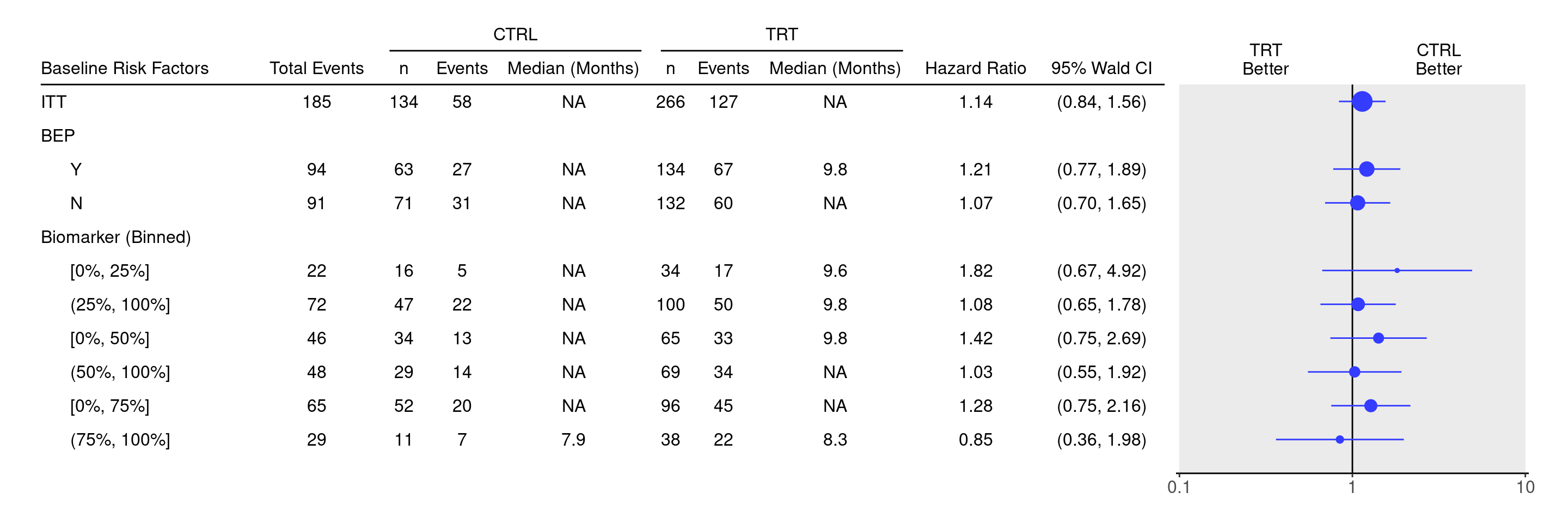
In this template we are looking for each percentage cutoff at above vs. below subgroups: So we just provide yet another groups_lists specification for the BMRKR1_BIN binned variable.

Code

BMRKR1_BIN_levels <- levels(adtte$BMRKR1_BIN)

tbl <- extract_survival_subgroups(
  variables = list(
    tte = "AVAL",
    is_event = "is_event",
    arm = "ARM_BIN",
    subgroups = c("BEP01FL", "BMRKR1_BIN")
  ),
  label_all = "ITT",
  groups_lists = list(
    BMRKR1_BIN = list(
      "[0%, 25%]" = BMRKR1_BIN_levels[1],
      "(25%, 100%]" = BMRKR1_BIN_levels[2:4],
      "[0%, 50%]" = BMRKR1_BIN_levels[1:2],
      "(50%, 100%]" = BMRKR1_BIN_levels[3:4],
      "[0%, 75%]" = BMRKR1_BIN_levels[1:3],
      "(75%, 100%]" = BMRKR1_BIN_levels[4]
    )
  ),
  data = adtte
)

result <- basic_table() %>%
  tabulate_survival_subgroups(
    df = tbl,
    vars = c("n_tot_events", "n", "n_events", "median", "hr", "ci"),
    time_unit = adtte$AVALU[1]
  )

We can now produce the forest plot using the g_forest() function.

Code

g_forest(result)

Code

sessionInfo()

R version 4.4.2 (2024-10-31)
Platform: x86_64-pc-linux-gnu
Running under: Ubuntu 24.04.1 LTS

Matrix products: default
BLAS:   /usr/lib/x86_64-linux-gnu/openblas-pthread/libblas.so.3 
LAPACK: /usr/lib/x86_64-linux-gnu/openblas-pthread/libopenblasp-r0.3.26.so;  LAPACK version 3.12.0

locale:
 [1] LC_CTYPE=en_US.UTF-8       LC_NUMERIC=C              
 [3] LC_TIME=en_US.UTF-8        LC_COLLATE=en_US.UTF-8    
 [5] LC_MONETARY=en_US.UTF-8    LC_MESSAGES=en_US.UTF-8   
 [7] LC_PAPER=en_US.UTF-8       LC_NAME=C                 
 [9] LC_ADDRESS=C               LC_TELEPHONE=C            
[11] LC_MEASUREMENT=en_US.UTF-8 LC_IDENTIFICATION=C       

time zone: Etc/UTC
tzcode source: system (glibc)

attached base packages:
[1] stats     graphics  grDevices utils     datasets  methods   base     

other attached packages:
[1] dplyr_1.1.4       tern_0.9.7        rtables_0.6.11    magrittr_2.0.3   
[5] formatters_0.5.10

loaded via a namespace (and not attached):
 [1] Matrix_1.7-2             gtable_0.3.6             jsonlite_1.9.0          
 [4] compiler_4.4.2           tidyselect_1.2.1         stringr_1.5.1           
 [7] tidyr_1.3.1              splines_4.4.2            scales_1.3.0            
[10] yaml_2.3.10              fastmap_1.2.0            lattice_0.22-6          
[13] ggplot2_3.5.1            R6_2.6.1                 labeling_0.4.3          
[16] generics_0.1.3           knitr_1.49               forcats_1.0.0           
[19] rbibutils_2.3            htmlwidgets_1.6.4        backports_1.5.0         
[22] checkmate_2.3.2          tibble_3.2.1             munsell_0.5.1           
[25] pillar_1.10.1            rlang_1.1.5              broom_1.0.7             
[28] stringi_1.8.4            xfun_0.51                cli_3.6.4               
[31] withr_3.0.2              Rdpack_2.6.2             digest_0.6.37           
[34] grid_4.4.2               cowplot_1.1.3            lifecycle_1.0.4         
[37] vctrs_0.6.5              evaluate_1.0.3           glue_1.8.0              
[40] farver_2.1.2             nestcolor_0.1.3          codetools_0.2-20        
[43] survival_3.8-3           random.cdisc.data_0.3.16 colorspace_2.1-1        
[46] rmarkdown_2.29           purrr_1.0.4              tools_4.4.2             
[49] pkgconfig_2.0.3          htmltools_0.5.8.1

Reuse