Biomarker Analysis Catalog - Stable
  • Stable
    • Dev
  1. Graphs
  2. SFG
  3. SFG4
  • Index

  • Tables
    • CPMT
      • CPMT1
      • CPMT2
        • CPMT2A
      • CPMT3
    • DT
      • DT1
        • DT1A
        • DT1B
        • DT1C
      • DT2
        • DT2A
    • TET
      • TET1
        • TET1A

  • Graphs
    • AG
      • AG1
    • DG
      • DG1
        • DG1A
        • DG1B
      • DG2
      • DG3
        • DG3A
      • DG4
    • KG
      • KG1
        • KG1A
        • KG1B
      • KG2
        • KG2A
      • KG3
      • KG4
        • KG4A
        • KG4B
      • KG5
        • KG5A
        • KG5B
    • RFG
      • RFG1
        • RFG1A
      • RFG2
        • RFG2A
        • RFG2B
        • RFG2C
      • RFG3
    • RG
      • RG1
        • RG1A
        • RG1B
        • RG1C
      • RG2
        • RG2A
      • RG3
        • RG3A
        • RG3B
    • SPG
      • SPG1
      • SPG2
    • RNAG
      • RNAG1
      • RNAG2
      • RNAG3
      • RNAG4
      • RNAG5
      • RNAG6
      • RNAG7
      • RNAG8
      • RNAG9
      • RNAG10
    • SFG
      • SFG1
        • SFG1A
        • SFG1B
      • SFG2
        • SFG2A
        • SFG2B
        • SFG2C
        • SFG2D
      • SFG3
        • SFG3A
      • SFG4
      • SFG5
        • SFG5A
        • SFG5B
        • SFG5C
      • SFG6
        • SFG6A
        • SFG6B
        • SFG6C
  1. Graphs
  2. SFG
  3. SFG4

SFG4

Survival Forest Graphs Within Treatment Arms by Continuous Biomarker Cutoff

SFG

  • Setup
  • Plot
  • Session Info

We prepare the data similarly as in SFG1.

Code
library(tern)
library(dplyr)

adtte <- random.cdisc.data::cadtte %>%
  df_explicit_na() %>%
  filter(
    PARAMCD == "OS",
    BEP01FL == "Y"
  ) %>%
  mutate(
    AVAL = day2month(AVAL),
    AVALU = "Months",
    is_event = CNSR == 0,
    ARM_BIN = fct_collapse_only(
      ARM,
      CTRL = "B: Placebo",
      TRT = c("A: Drug X", "C: Combination")
    )
  ) %>%
  var_relabel(
    BEP01FL = "BEP",
    BMRKR1 = "Biomarker (Countinuous)"
  )

We define a vector of all cutpoints to use for a numeric biomarker (here BMRKR1). We lapply() over this vector, each time generating a binary factor variable BMRKR1_cut and then tabulating the resulting statistics similar to SFG3, this time including the treatment arms in the subgroups argument. Then we rbind() all tables in the list together.

Code
all_cutpoints <- c(2.5, 5, 7.5, 10)

tables_all_cutpoints <- lapply(all_cutpoints, function(cutpoint) {
  adtte_cut <- adtte %>%
    mutate(
      BMRKR1_cut = explicit_na(factor(
        ifelse(BMRKR1 > cutpoint, "Greater", "Less")
      ))
    )
  tbl <- extract_survival_subgroups(
    variables = list(
      tte = "AVAL",
      is_event = "is_event",
      arm = "BMRKR1_cut",
      subgroups = "ARM_BIN"
    ),
    label_all = paste0("BMRKR1 (", cutpoint, ")"),
    data = adtte_cut
  )
  basic_table() %>%
    tabulate_survival_subgroups(
      df = tbl,
      vars = c("n_tot_events", "n", "n_events", "median", "hr", "ci"),
      time_unit = adtte_cut$AVALU[1]
    )
})

result <- do.call(rbind, tables_all_cutpoints)

We can now produce the forest plot using the g_forest() function. Similarly as in SFG3 we need to specify the col_x, col_y and forest_header arguments for g_forest() by recovering them from one of the original tables.

Code
one_table <- tables_all_cutpoints[[1]]
g_forest(
  result,
  col_x = attr(one_table, "col_x"),
  col_ci = attr(one_table, "col_ci"),
  forest_header = attr(one_table, "forest_header"),
  col_symbol_size = attr(one_table, "col_symbol_size")
)

Code
sessionInfo()
R version 4.4.2 (2024-10-31)
Platform: x86_64-pc-linux-gnu
Running under: Ubuntu 24.04.1 LTS

Matrix products: default
BLAS:   /usr/lib/x86_64-linux-gnu/openblas-pthread/libblas.so.3 
LAPACK: /usr/lib/x86_64-linux-gnu/openblas-pthread/libopenblasp-r0.3.26.so;  LAPACK version 3.12.0

locale:
 [1] LC_CTYPE=en_US.UTF-8       LC_NUMERIC=C              
 [3] LC_TIME=en_US.UTF-8        LC_COLLATE=en_US.UTF-8    
 [5] LC_MONETARY=en_US.UTF-8    LC_MESSAGES=en_US.UTF-8   
 [7] LC_PAPER=en_US.UTF-8       LC_NAME=C                 
 [9] LC_ADDRESS=C               LC_TELEPHONE=C            
[11] LC_MEASUREMENT=en_US.UTF-8 LC_IDENTIFICATION=C       

time zone: Etc/UTC
tzcode source: system (glibc)

attached base packages:
[1] stats     graphics  grDevices utils     datasets  methods   base     

other attached packages:
[1] dplyr_1.1.4       tern_0.9.7        rtables_0.6.11    magrittr_2.0.3   
[5] formatters_0.5.10

loaded via a namespace (and not attached):
 [1] Matrix_1.7-2             gtable_0.3.6             jsonlite_1.9.0          
 [4] compiler_4.4.2           tidyselect_1.2.1         stringr_1.5.1           
 [7] tidyr_1.3.1              splines_4.4.2            scales_1.3.0            
[10] yaml_2.3.10              fastmap_1.2.0            lattice_0.22-6          
[13] ggplot2_3.5.1            R6_2.6.1                 labeling_0.4.3          
[16] generics_0.1.3           knitr_1.49               forcats_1.0.0           
[19] rbibutils_2.3            htmlwidgets_1.6.4        backports_1.5.0         
[22] checkmate_2.3.2          tibble_3.2.1             munsell_0.5.1           
[25] pillar_1.10.1            rlang_1.1.5              broom_1.0.7             
[28] stringi_1.8.4            xfun_0.51                cli_3.6.4               
[31] withr_3.0.2              Rdpack_2.6.2             digest_0.6.37           
[34] grid_4.4.2               cowplot_1.1.3            lifecycle_1.0.4         
[37] vctrs_0.6.5              evaluate_1.0.3           glue_1.8.0              
[40] farver_2.1.2             nestcolor_0.1.3          codetools_0.2-20        
[43] survival_3.8-3           random.cdisc.data_0.3.16 colorspace_2.1-1        
[46] rmarkdown_2.29           purrr_1.0.4              tools_4.4.2             
[49] pkgconfig_2.0.3          htmltools_0.5.8.1       

Reuse

Copyright 2023, Hoffmann-La Roche Ltd.
SFG3A
SFG5
Source Code
---
title: SFG4
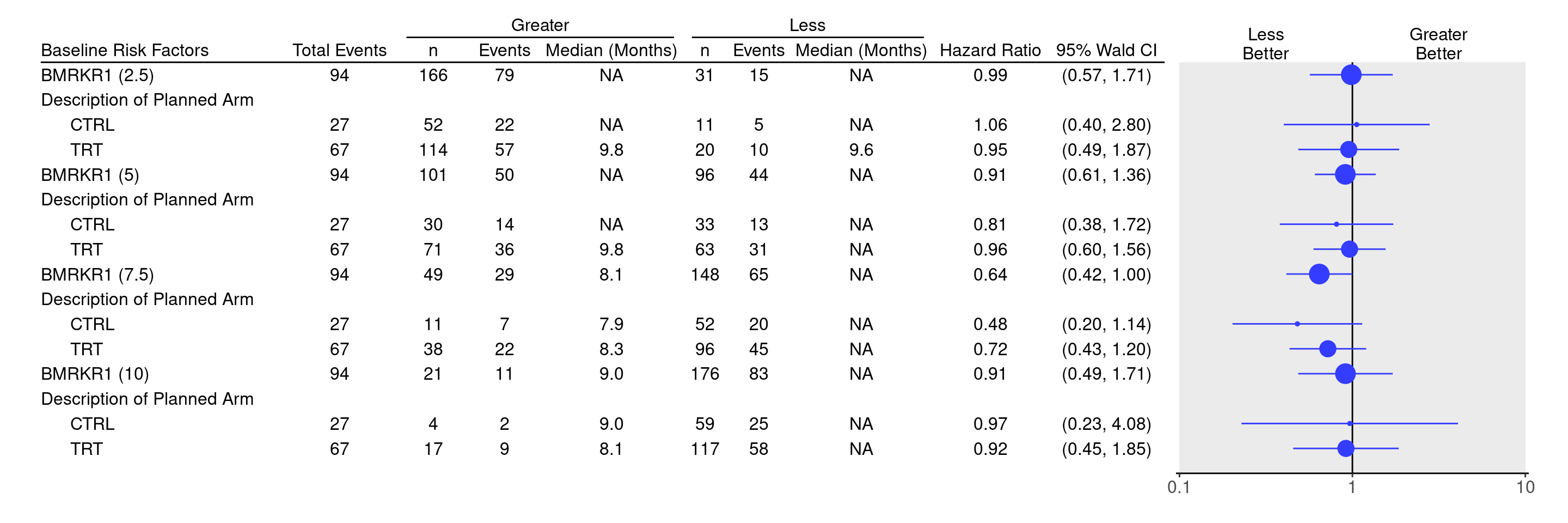
subtitle: Survival Forest Graphs Within Treatment Arms by Continuous Biomarker Cutoff
categories: [SFG]
---

------------------------------------------------------------------------

::: panel-tabset
## Setup

We prepare the data similarly as in [SFG1](../graphs/SFG1/sfg01.qmd).

```{r, message = FALSE}
library(tern)
library(dplyr)

adtte <- random.cdisc.data::cadtte %>%
  df_explicit_na() %>%
  filter(
    PARAMCD == "OS",
    BEP01FL == "Y"
  ) %>%
  mutate(
    AVAL = day2month(AVAL),
    AVALU = "Months",
    is_event = CNSR == 0,
    ARM_BIN = fct_collapse_only(
      ARM,
      CTRL = "B: Placebo",
      TRT = c("A: Drug X", "C: Combination")
    )
  ) %>%
  var_relabel(
    BEP01FL = "BEP",
    BMRKR1 = "Biomarker (Countinuous)"
  )
```

## Plot

We define a vector of all cutpoints to use for a numeric biomarker (here `BMRKR1`).
We `lapply()` over this vector, each time generating a binary factor variable `BMRKR1_cut` and then tabulating the resulting statistics similar to [SFG3](../graphs/SFG3/sfg03.qmd), this time including the treatment arms in the `subgroups` argument.
Then we `rbind()` all tables in the list together.

```{r}
all_cutpoints <- c(2.5, 5, 7.5, 10)

tables_all_cutpoints <- lapply(all_cutpoints, function(cutpoint) {
  adtte_cut <- adtte %>%
    mutate(
      BMRKR1_cut = explicit_na(factor(
        ifelse(BMRKR1 > cutpoint, "Greater", "Less")
      ))
    )
  tbl <- extract_survival_subgroups(
    variables = list(
      tte = "AVAL",
      is_event = "is_event",
      arm = "BMRKR1_cut",
      subgroups = "ARM_BIN"
    ),
    label_all = paste0("BMRKR1 (", cutpoint, ")"),
    data = adtte_cut
  )
  basic_table() %>%
    tabulate_survival_subgroups(
      df = tbl,
      vars = c("n_tot_events", "n", "n_events", "median", "hr", "ci"),
      time_unit = adtte_cut$AVALU[1]
    )
})

result <- do.call(rbind, tables_all_cutpoints)
```

We can now produce the forest plot using the `g_forest()` function.
Similarly as in [SFG3](../graphs/SFG3/sfg03.qmd) we need to specify the `col_x`, `col_y` and `forest_header` arguments for `g_forest()` by recovering them from one of the original tables.

```{r, fig.width = 15}
one_table <- tables_all_cutpoints[[1]]
g_forest(
  result,
  col_x = attr(one_table, "col_x"),
  col_ci = attr(one_table, "col_ci"),
  forest_header = attr(one_table, "forest_header"),
  col_symbol_size = attr(one_table, "col_symbol_size")
)
```

{{< include ../misc/session_info.qmd >}}
:::

Made with ❤️ by the Statistical Engineering Team StatisticalEngineering

  • License

  • Edit this page
  • Report an issue
Cookie Preferences