RNAG9

RNAseq Kaplan-Meier Graph

RNAG

This page can be used as a template of how to produce Kaplan-Meier graphs for RNA-seq gene expression analysis using available tern and hermes functions, and to create an interactive Kaplan-Meier graph for RNA-seq gene expression analysis using teal.modules.hermes.

The code below needs both RNA-seq data (in HermesData format) and time-to-event data (in ADTTE format) as input.

We first prepare the time-to-event data. We define an event indicator variable, transform the time to months and filter down to the overall survival subset.

Code

library(tern)
library(dplyr)

adtte_f <- random.cdisc.data::cadtte %>%
  dplyr::mutate(
    is_event = .data$CNSR == 0,
    AVAL = day2month(.data$AVAL),
    AVALU = "Months"
  ) %>%
  dplyr::filter(.data$PARAMCD == "OS")

Then we prepare the RNA-seq data. See RNAG1 for basic details on how to import, filter and normalize HermesData. We use col_data_with_genes() to extract the sample variables (colData) from the object, together with a single specified gene or a specified gene signature. See ?hermes::gene_spec for details on how to do this. Then we use inner_join_cdisc() to join this genetic data with the ADTTE data from above. See the help page for more details, in particular how the join keys can be customized if needed - here we just join based on USUBJID by default.

Code

library(hermes)

gene_data <- col_data_with_genes(
  object = hermes_data,
  assay_name = "counts",
  genes = gene_spec("GeneID:1820")
)
joined_data <- inner_join_cdisc(
  gene_data = gene_data,
  cdisc_data = adtte_f
)

We can then cut the resulting gene column (we figure out the column name and save it in arm_name below) in the joined_data into quantile bins (in this example we want three equally sized groups).

Code

arm_name <- attr(gene_data, "gene_cols")
binned_data <- joined_data %>%
  dplyr::mutate(
    gene_factor = cut_quantile_bins(
      joined_data[[arm_name]],
      probs = c(1 / 3, 2 / 3)
    )
  ) %>%
  df_explicit_na()

It is now simple to create the Kaplan-Meier graph by providing the data set created above with the variable specification. Note that we specify the above created gene_factor as arm variable here.

Code

variables <- list(
  tte = "AVAL",
  is_event = "is_event",
  arm = "gene_factor"
)
g_km(
  binned_data,
  variables = variables,
  annot_coxph = TRUE
)

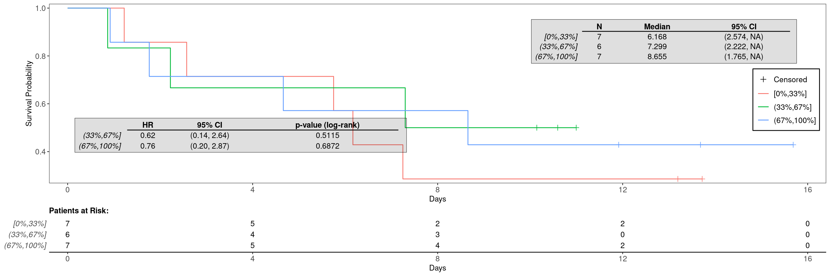
See KG1 to KG5 for additional customization options for the Kaplan-Meier graphs or the help page ?g_km().

We start by importing a MultiAssayExperiment and sample ADTTE data; here we use the example multi_assay_experiment available in hermes and example ADTTE data from random.cdisc.data. We can then use the provided teal module tm_g_km to include the corresponding interactive Kaplan-Meier analysis in our teal app. Note that by default the counts assay is excluded via the exclude_assays argument, but we can include it by just saying that we don’t want to exclude any assays. In case that we have different non-standard column names in our ADTTE data set we could also specify them via the adtte_vars argument, see the documentation ?tm_g_km for more details.

Code

library(teal.modules.hermes)

data <- teal_data()
data <- within(data, {
  library(random.cdisc.data)
  library(dplyr)
  library(hermes)
  MAE <- multi_assay_experiment
  ADTTE <- random.cdisc.data::cadtte %>%
    mutate(is_event = .data$CNSR == 0)
})
datanames(data) <- c("MAE", "ADTTE")

Warning: `datanames<-()` was deprecated in teal.data 0.7.0.
ℹ invalid to use `datanames()<-` or `names()<-` on an object of class
  `teal_data`. See ?names.teal_data

Code

join_keys(data)["ADTTE", "ADTTE"] <- c("STUDYID", "USUBJID", "PARAMCD")

app <- init(
  data = data,
  modules = modules(
    tm_g_km(
      label = "Kaplan-Meier Graph",
      adtte_name = "ADTTE",
      mae_name = "MAE",
      exclude_assays = character()
    )
  )
)

[INFO] 2025-02-19 17:26:28.7126 pid:3180 token:[] teal.modules.hermes Initializing tm_g_km

Code

shinyApp(app$ui, app$server)

Warning: 'experiments' dropped; see 'drops()'

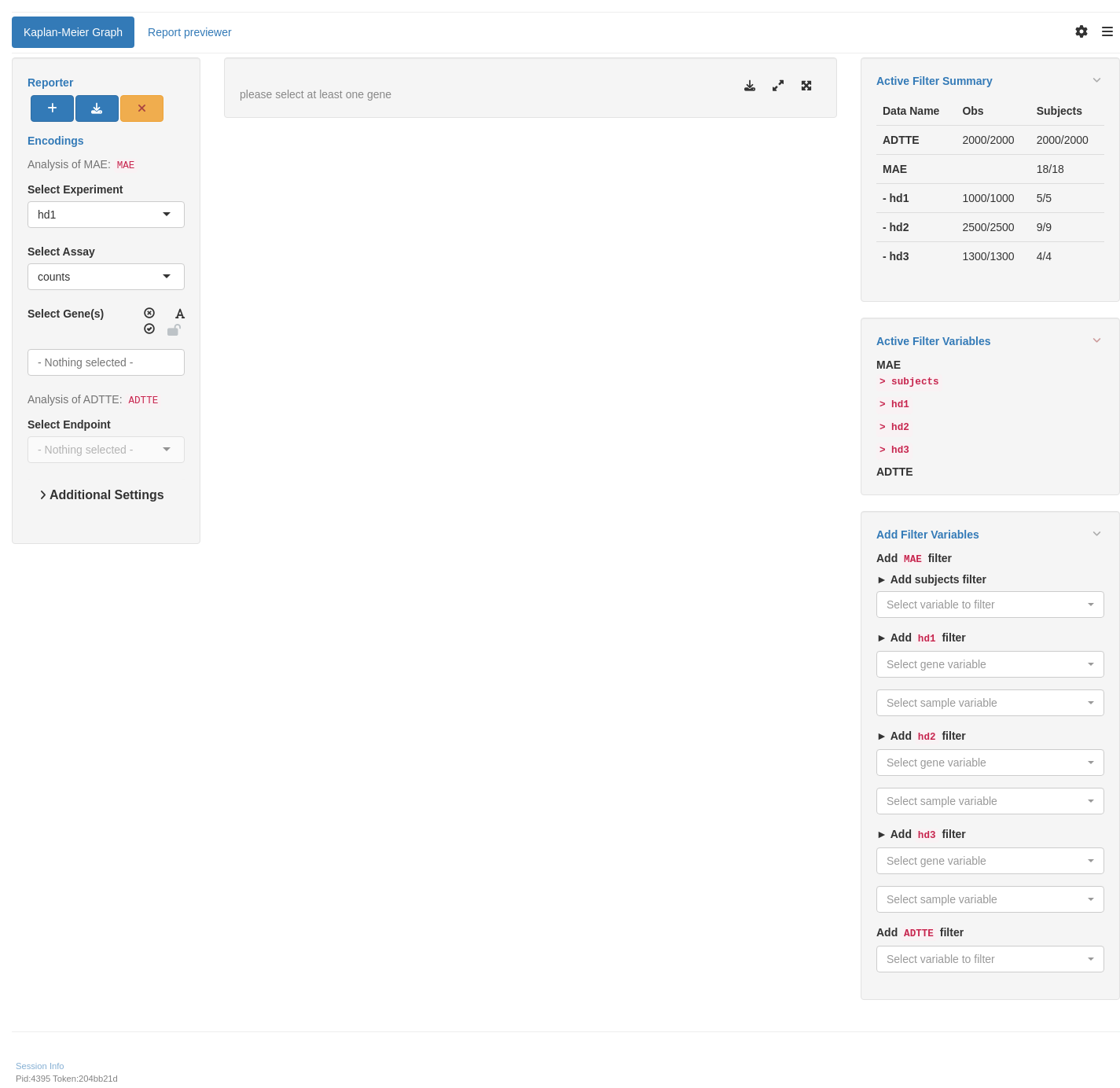
Code

sessionInfo()

R version 4.4.2 (2024-10-31)
Platform: x86_64-pc-linux-gnu
Running under: Ubuntu 24.04.1 LTS

Matrix products: default
BLAS:   /usr/lib/x86_64-linux-gnu/openblas-pthread/libblas.so.3 
LAPACK: /usr/lib/x86_64-linux-gnu/openblas-pthread/libopenblasp-r0.3.26.so;  LAPACK version 3.12.0

locale:
 [1] LC_CTYPE=en_US.UTF-8       LC_NUMERIC=C              
 [3] LC_TIME=en_US.UTF-8        LC_COLLATE=en_US.UTF-8    
 [5] LC_MONETARY=en_US.UTF-8    LC_MESSAGES=en_US.UTF-8   
 [7] LC_PAPER=en_US.UTF-8       LC_NAME=C                 
 [9] LC_ADDRESS=C               LC_TELEPHONE=C            
[11] LC_MEASUREMENT=en_US.UTF-8 LC_IDENTIFICATION=C       

time zone: Etc/UTC
tzcode source: system (glibc)

attached base packages:
[1] stats4    stats     graphics  grDevices utils     datasets  methods  
[8] base     

other attached packages:
 [1] random.cdisc.data_0.3.16    teal.modules.hermes_0.1.6  
 [3] teal_0.16.0                 teal.slice_0.6.0           
 [5] teal.data_0.7.0             teal.code_0.6.1            
 [7] shiny_1.10.0                hermes_1.10.0              
 [9] SummarizedExperiment_1.36.0 Biobase_2.66.0             
[11] GenomicRanges_1.58.0        GenomeInfoDb_1.42.3        
[13] IRanges_2.40.1              S4Vectors_0.44.0           
[15] BiocGenerics_0.52.0         MatrixGenerics_1.18.1      
[17] matrixStats_1.5.0           ggfortify_0.4.17           
[19] ggplot2_3.5.1               dplyr_1.1.4                
[21] tern_0.9.7                  rtables_0.6.11             
[23] magrittr_2.0.3              formatters_0.5.10          

loaded via a namespace (and not attached):
  [1] RColorBrewer_1.1-3          jsonlite_1.9.0             
  [3] shape_1.4.6.1               nestcolor_0.1.3            
  [5] MultiAssayExperiment_1.32.0 farver_2.1.2               
  [7] rmarkdown_2.29              GlobalOptions_0.1.2        
  [9] zlibbioc_1.52.0             vctrs_0.6.5                
 [11] memoise_2.0.1               webshot_0.5.5              
 [13] BiocBaseUtils_1.9.0         htmltools_0.5.8.1          
 [15] S4Arrays_1.6.0              forcats_1.0.0              
 [17] progress_1.2.3              curl_6.2.1                 
 [19] broom_1.0.7                 SparseArray_1.6.1          
 [21] sass_0.4.9                  bslib_0.9.0                
 [23] fontawesome_0.5.3           htmlwidgets_1.6.4          
 [25] httr2_1.1.0                 cachem_1.1.0               
 [27] teal.widgets_0.4.3          mime_0.12                  
 [29] lifecycle_1.0.4             iterators_1.0.14           
 [31] pkgconfig_2.0.3             webshot2_0.1.1             
 [33] Matrix_1.7-2                R6_2.6.1                   
 [35] fastmap_1.2.0               GenomeInfoDbData_1.2.13    
 [37] rbibutils_2.3               clue_0.3-66                
 [39] digest_0.6.37               colorspace_2.1-1           
 [41] shinycssloaders_1.1.0       ps_1.9.0                   
 [43] AnnotationDbi_1.68.0        RSQLite_2.3.9              
 [45] filelock_1.0.3              labeling_0.4.3             
 [47] httr_1.4.7                  abind_1.4-8                
 [49] compiler_4.4.2              bit64_4.6.0-1              
 [51] withr_3.0.2                 doParallel_1.0.17          
 [53] backports_1.5.0             DBI_1.2.3                  
 [55] logger_0.4.0                biomaRt_2.62.1             
 [57] rappdirs_0.3.3              DelayedArray_0.32.0        
 [59] rjson_0.2.23                chromote_0.4.0             
 [61] tools_4.4.2                 httpuv_1.6.15              
 [63] glue_1.8.0                  callr_3.7.6                
 [65] promises_1.3.2              grid_4.4.2                 
 [67] checkmate_2.3.2             cluster_2.1.8              
 [69] generics_0.1.3              gtable_0.3.6               
 [71] websocket_1.4.2             tidyr_1.3.1                
 [73] hms_1.1.3                   xml2_1.3.6                 
 [75] XVector_0.46.0              ggrepel_0.9.6              
 [77] foreach_1.5.2               pillar_1.10.1              
 [79] stringr_1.5.1               later_1.4.1                
 [81] circlize_0.4.16             splines_4.4.2              
 [83] BiocFileCache_2.14.0        lattice_0.22-6             
 [85] survival_3.8-3              bit_4.5.0.1                
 [87] tidyselect_1.2.1            ComplexHeatmap_2.22.0      
 [89] Biostrings_2.74.1           knitr_1.49                 
 [91] gridExtra_2.3               teal.logger_0.3.2          
 [93] xfun_0.51                   stringi_1.8.4              
 [95] UCSC.utils_1.2.0            yaml_2.3.10                
 [97] shinyWidgets_0.8.7          evaluate_1.0.3             
 [99] codetools_0.2-20            tibble_3.2.1               
[101] cli_3.6.4                   xtable_1.8-4               
[103] Rdpack_2.6.2                jquerylib_0.1.4            
[105] processx_3.8.5              munsell_0.5.1              
[107] teal.reporter_0.4.0         Rcpp_1.0.14                
[109] dbplyr_2.5.0                png_0.1-8                  
[111] parallel_4.4.2              assertthat_0.2.1           
[113] blob_1.2.4                  prettyunits_1.2.0          
[115] scales_1.3.0                purrr_1.0.4                
[117] crayon_1.5.3                GetoptLong_1.0.5           
[119] rlang_1.1.5                 formatR_1.14               
[121] cowplot_1.1.3               KEGGREST_1.46.0            
[123] shinyjs_2.1.0

Reuse