KG4

Kaplan-Meier Graphs by Treatment Arm and Biomarker Subgroups

A setup similar to KG1 is used, with some additional data manipulation steps to first binarize the continuous biomarker and the treatment arm variables, and then combine both into a new interaction variable ARM_BMRKR2. Since we are using biomarker information, we filter on the biomarker evaluable population using the flag variable BEP01FL.

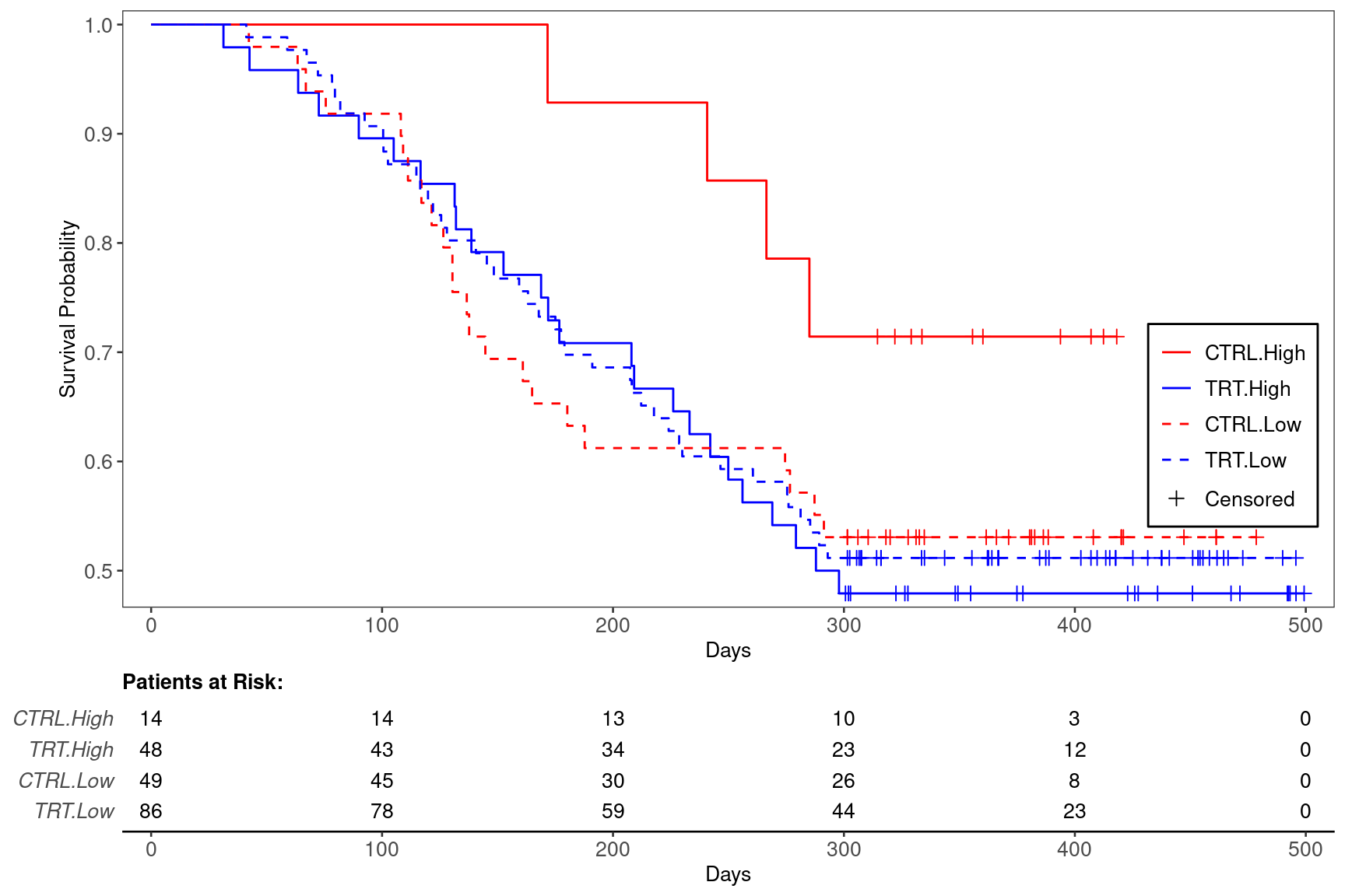
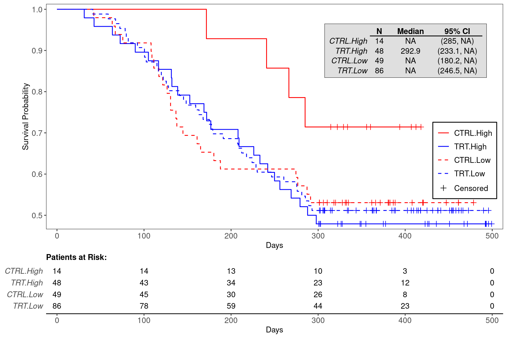
Code

library(tern)
library(dplyr)

adtte <- random.cdisc.data::cadtte %>%
  df_explicit_na() %>%
  filter(PARAMCD == "OS" & BEP01FL == "Y") %>%
  mutate(
    is_event = CNSR == 0,
    BMRKR2_BIN = fct_collapse_only(
      BMRKR2,
      High = c("HIGH"),
      Low = c("MEDIUM", "LOW")
    ),
    ARM_BIN = fct_collapse_only(
      ARM,
      CTRL = c("B: Placebo"),
      TRT = c("A: Drug X", "C: Combination")
    ),
    ARM_BMRKR2 = interaction(ARM_BIN, BMRKR2_BIN)
  )

variables <- list(tte = "AVAL", is_event = "is_event", arm = "ARM_BMRKR2")

We can produce the basic graph using the g_km() function from tern.

Code

g_km(
  df = adtte,
  variables = variables,
  annot_surv_med = FALSE,
  col = c("red", "blue", "red", "blue"),
  lty = c(1, 1, 2, 2)
)

We can also choose to annotate the plot with the median survival time for each of the treatment arms using the annot_surv_med = TRUE option.

Code

g_km(
  df = adtte,
  variables = variables,
  annot_surv_med = TRUE,
  col = c("red", "blue", "red", "blue"),
  lty = c(1, 1, 2, 2)
)

Code

sessionInfo()

R version 4.5.2 (2025-10-31)
Platform: x86_64-pc-linux-gnu
Running under: Ubuntu 24.04.4 LTS

Matrix products: default
BLAS:   /usr/lib/x86_64-linux-gnu/openblas-pthread/libblas.so.3 
LAPACK: /usr/lib/x86_64-linux-gnu/openblas-pthread/libopenblasp-r0.3.26.so;  LAPACK version 3.12.0

locale:
 [1] LC_CTYPE=en_US.UTF-8       LC_NUMERIC=C              
 [3] LC_TIME=en_US.UTF-8        LC_COLLATE=en_US.UTF-8    
 [5] LC_MONETARY=en_US.UTF-8    LC_MESSAGES=en_US.UTF-8   
 [7] LC_PAPER=en_US.UTF-8       LC_NAME=C                 
 [9] LC_ADDRESS=C               LC_TELEPHONE=C            
[11] LC_MEASUREMENT=en_US.UTF-8 LC_IDENTIFICATION=C       

time zone: Etc/UTC
tzcode source: system (glibc)

attached base packages:
[1] stats     graphics  grDevices utils     datasets  methods   base     

other attached packages:
[1] dplyr_1.2.1       tern_0.9.10       rtables_0.6.15    magrittr_2.0.5   
[5] formatters_0.5.12

loaded via a namespace (and not attached):
 [1] generics_0.1.4           tidyr_1.3.2              stringi_1.8.7           
 [4] lattice_0.22-9           digest_0.6.39            evaluate_1.0.5          
 [7] grid_4.5.2               RColorBrewer_1.1-3       fastmap_1.2.0           
[10] jsonlite_2.0.0           Matrix_1.7-5             backports_1.5.1         
[13] survival_3.8-6           purrr_1.2.1              scales_1.4.0            
[16] codetools_0.2-20         Rdpack_2.6.6             cli_3.6.5               
[19] nestcolor_0.1.3          rlang_1.2.0              rbibutils_2.4.1         
[22] cowplot_1.2.0            splines_4.5.2            withr_3.0.2             
[25] yaml_2.3.12              otel_0.2.0               tools_4.5.2             
[28] checkmate_2.3.4          ggplot2_4.0.2            forcats_1.0.1           
[31] broom_1.0.12             vctrs_0.7.2              R6_2.6.1                
[34] lifecycle_1.0.5          stringr_1.6.0            htmlwidgets_1.6.4       
[37] pkgconfig_2.0.3          pillar_1.11.1            gtable_0.3.6            
[40] glue_1.8.0               xfun_0.57                tibble_3.3.1            
[43] tidyselect_1.2.1         knitr_1.51               dichromat_2.0-0.1       
[46] farver_2.1.2             htmltools_0.5.9          rmarkdown_2.31          
[49] labeling_0.4.3           random.cdisc.data_0.3.16 compiler_4.5.2          
[52] S7_0.2.1

Reuse