RNAG4

RNAseq Sample Correlation Graph

---

Setup: Import, Filter and Normalize

This page can be used as a template of how to use the available hermes functions to calculate the correlation between samples in HermesData, visualize them in a heatmap, and create an interactive sample correlation graph using teal.modules.hermes.

The function used to calculate correlation uses HermesData as input. See RNAG1 for details.

library(hermes)

object <- hermes_data %>%
  add_quality_flags() %>%
  filter() %>%
  normalize()

Calculate Correlation

We can calculate correlation matrix between samples in HermesData using correlate() function. By default, correlate() function uses the counts assay to calculate the Pearson correlation coefficients, unless specified otherwise in the arguments.

result <- correlate(object)

result <- correlate(object, assay_name = "tpm", method = "spearman")

Plot Correlation

We can then plot a heatmap for correlation between samples in HermesData using the autoplot() function. See ?calc_cor for details.

autoplot(result)

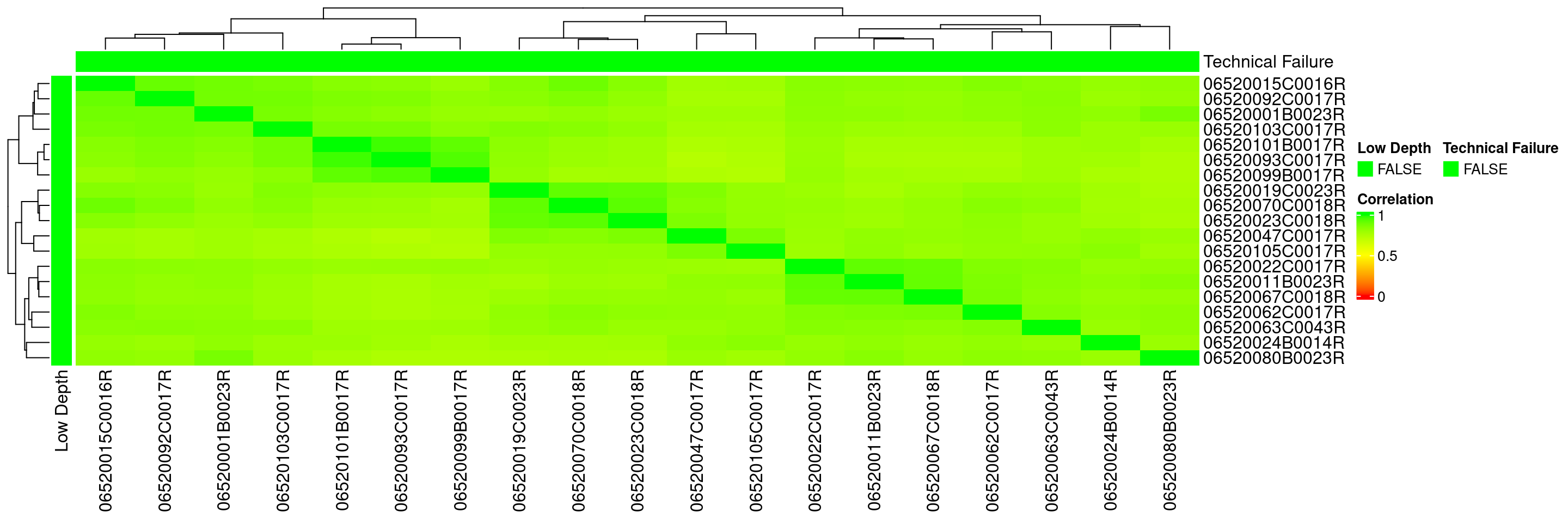
If there are still (because we already filtered some samples above) samples that have low correlation with others, we might want to flag them manually as technical failures and filter again. Here just as an example:

object <- object %>%
  set_tech_failure("06520011B0023R") %>%
  filter()

Teal Module for Sample Correlation Graph

We start by importing a MultiAssayExperiment; here we use the example multi_assay_experiment available in hermes. It is wrapped as a teal::dataset. We can select the sample correlation tab above the plot area. We can then use the provided teal module tm_g_pca to include a PCA module in our teal app.

library(teal.modules.hermes)

data <- teal_data()
data <- within(data, {
  library(hermes)
  MAE <- multi_assay_experiment
})
datanames(data) <- "MAE"

Warning: `datanames<-()` was deprecated in teal.data 0.7.0.
ℹ invalid to use `datanames()<-` or `names()<-` on an object of class
  `teal_data`. See ?names.teal_data

app <- init(
  data = data,
  modules = modules(
    tm_g_pca(
      label = "pca",
      mae_name = "MAE"
    )
  )
)

[INFO] 2025-02-19 17:31:12.1917 pid:6519 token:[] teal.modules.hermes Initializing tm_g_pca

shinyApp(app$ui, app$server)

Warning: 'experiments' dropped; see 'drops()'

Session Info

sessionInfo()

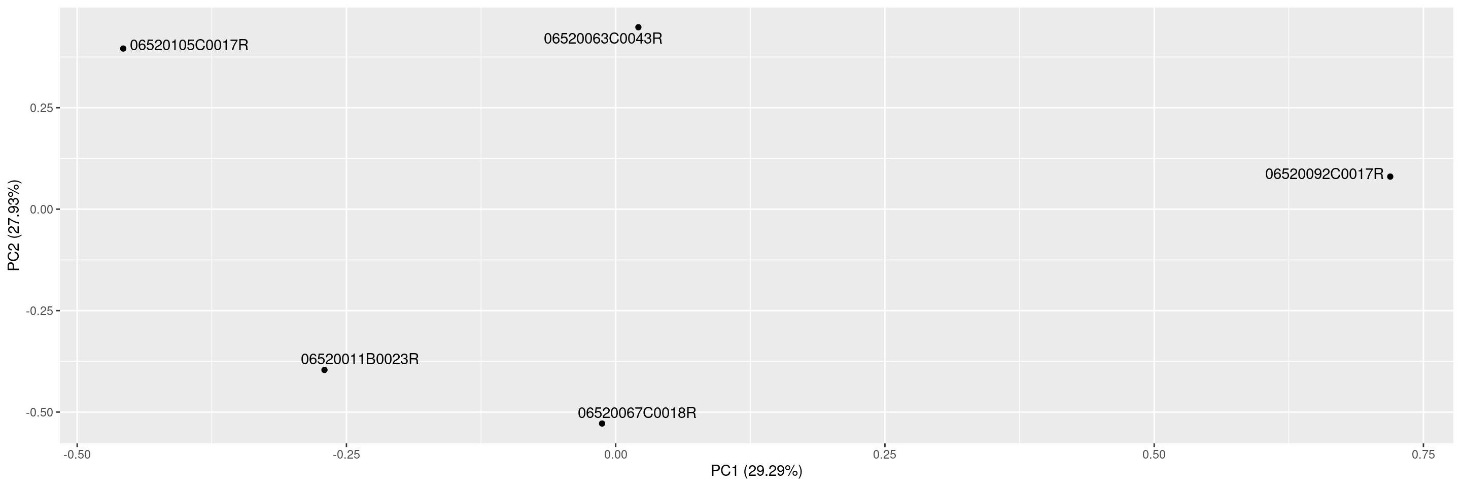
R version 4.4.2 (2024-10-31)
Platform: x86_64-pc-linux-gnu
Running under: Ubuntu 24.04.1 LTS

Matrix products: default
BLAS:   /usr/lib/x86_64-linux-gnu/openblas-pthread/libblas.so.3 
LAPACK: /usr/lib/x86_64-linux-gnu/openblas-pthread/libopenblasp-r0.3.26.so;  LAPACK version 3.12.0

locale:
 [1] LC_CTYPE=en_US.UTF-8       LC_NUMERIC=C              
 [3] LC_TIME=en_US.UTF-8        LC_COLLATE=en_US.UTF-8    
 [5] LC_MONETARY=en_US.UTF-8    LC_MESSAGES=en_US.UTF-8   
 [7] LC_PAPER=en_US.UTF-8       LC_NAME=C                 
 [9] LC_ADDRESS=C               LC_TELEPHONE=C            
[11] LC_MEASUREMENT=en_US.UTF-8 LC_IDENTIFICATION=C       

time zone: Etc/UTC
tzcode source: system (glibc)

attached base packages:
[1] stats4    stats     graphics  grDevices utils     datasets  methods  
[8] base     

other attached packages:
 [1] teal.modules.hermes_0.1.6   teal_0.16.0                
 [3] teal.slice_0.6.0            teal.data_0.7.0            
 [5] teal.code_0.6.1             shiny_1.10.0               
 [7] hermes_1.10.0               SummarizedExperiment_1.36.0
 [9] Biobase_2.66.0              GenomicRanges_1.58.0       
[11] GenomeInfoDb_1.42.3         IRanges_2.40.1             
[13] S4Vectors_0.44.0            BiocGenerics_0.52.0        
[15] MatrixGenerics_1.18.1       matrixStats_1.5.0          
[17] ggfortify_0.4.17            ggplot2_3.5.1              

loaded via a namespace (and not attached):
  [1] RColorBrewer_1.1-3          jsonlite_1.9.0             
  [3] shape_1.4.6.1               MultiAssayExperiment_1.32.0
  [5] magrittr_2.0.3              magick_2.8.5               
  [7] farver_2.1.2                rmarkdown_2.29             
  [9] ragg_1.3.3                  GlobalOptions_0.1.2        
 [11] zlibbioc_1.52.0             vctrs_0.6.5                
 [13] memoise_2.0.1               webshot_0.5.5              
 [15] BiocBaseUtils_1.9.0         htmltools_0.5.8.1          
 [17] S4Arrays_1.6.0              forcats_1.0.0              
 [19] progress_1.2.3              curl_6.2.1                 
 [21] SparseArray_1.6.1           sass_0.4.9                 
 [23] bslib_0.9.0                 fontawesome_0.5.3          
 [25] htmlwidgets_1.6.4           testthat_3.2.3             
 [27] httr2_1.1.0                 cachem_1.1.0               
 [29] teal.widgets_0.4.3          mime_0.12                  
 [31] lifecycle_1.0.4             iterators_1.0.14           
 [33] pkgconfig_2.0.3             webshot2_0.1.1             
 [35] Matrix_1.7-2                R6_2.6.1                   
 [37] fastmap_1.2.0               GenomeInfoDbData_1.2.13    
 [39] rbibutils_2.3               clue_0.3-66                
 [41] digest_0.6.37               colorspace_2.1-1           
 [43] shinycssloaders_1.1.0       AnnotationDbi_1.68.0       
 [45] ps_1.9.0                    DESeq2_1.46.0              
 [47] textshaping_1.0.0           crosstalk_1.2.1            
 [49] RSQLite_2.3.9               labeling_0.4.3             
 [51] filelock_1.0.3              httr_1.4.7                 
 [53] abind_1.4-8                 compiler_4.4.2             
 [55] bit64_4.6.0-1               withr_3.0.2                
 [57] doParallel_1.0.17           backports_1.5.0            
 [59] BiocParallel_1.40.0         DBI_1.2.3                  
 [61] logger_0.4.0                biomaRt_2.62.1             
 [63] rappdirs_0.3.3              DelayedArray_0.32.0        
 [65] rjson_0.2.23                tools_4.4.2                
 [67] chromote_0.4.0              httpuv_1.6.15              
 [69] glue_1.8.0                  callr_3.7.6                
 [71] promises_1.3.2              grid_4.4.2                 
 [73] checkmate_2.3.2             cluster_2.1.8              
 [75] generics_0.1.3              gtable_0.3.6               
 [77] websocket_1.4.2             tidyr_1.3.1                
 [79] hms_1.1.3                   xml2_1.3.6                 
 [81] XVector_0.46.0              ggrepel_0.9.6              
 [83] foreach_1.5.2               pillar_1.10.1              
 [85] stringr_1.5.1               limma_3.62.2               
 [87] later_1.4.1                 circlize_0.4.16            
 [89] dplyr_1.1.4                 BiocFileCache_2.14.0       
 [91] lattice_0.22-6              bit_4.5.0.1                
 [93] tidyselect_1.2.1            ComplexHeatmap_2.22.0      
 [95] locfit_1.5-9.11             Biostrings_2.74.1          
 [97] knitr_1.49                  gridExtra_2.3              
 [99] teal.logger_0.3.2           edgeR_4.4.2                
[101] xfun_0.51                   statmod_1.5.0              
[103] brio_1.1.5                  DT_0.33                    
[105] stringi_1.8.4               UCSC.utils_1.2.0           
[107] yaml_2.3.10                 shinyWidgets_0.8.7         
[109] evaluate_1.0.3              codetools_0.2-20           
[111] tibble_3.2.1                cli_3.6.4                  
[113] systemfonts_1.2.1           xtable_1.8-4               
[115] Rdpack_2.6.2                jquerylib_0.1.4            
[117] munsell_0.5.1               processx_3.8.5             
[119] teal.reporter_0.4.0         Rcpp_1.0.14                
[121] dbplyr_2.5.0                png_0.1-8                  
[123] parallel_4.4.2              assertthat_0.2.1           
[125] blob_1.2.4                  prettyunits_1.2.0          
[127] scales_1.3.0                purrr_1.0.4                
[129] crayon_1.5.3                GetoptLong_1.0.5           
[131] rlang_1.1.5                 formatR_1.14               
[133] KEGGREST_1.46.0             shinyjs_2.1.0