KG1A

Kaplan-Meier Graph for Biomarker Evaluable Population in One Treatment Arm

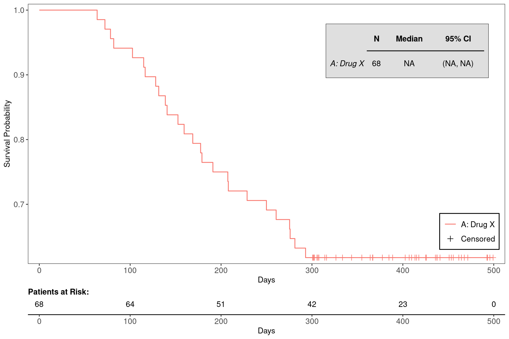
We will use the cadtte data set from the random.cdisc.data package to create the Kaplan-Meier (KM) plots. We start by filtering the time-to-event dataset for the overall survival observations and by one treatment arm (A), creating a new variable for event information, and curating a list of variables required to produce the plot.

Code

library(tern)
library(dplyr)
library(ggplot2)
library(grid)

adtte_arm <- random.cdisc.data::cadtte %>%
  df_explicit_na() %>%
  filter(PARAMCD == "OS", ARM == "A: Drug X") %>%
  mutate(is_event = CNSR == 0)

variables <- list(tte = "AVAL", is_event = "is_event", arm = "ARM")

We can filter the dataset further for the biomarker evaluable population using the corresponding flag variable, here BEP01FL:

Code

adtte_arm_bep <- adtte_arm %>%
  filter(BEP01FL == "Y")

Afterwards we can plot the basic KM graph, just using the further filtered dataset adtte_bep. Here we annotate the plot with median survival time, but could suppress it with annot_surv_med = FALSE.

Code

g_km(
  df = adtte_arm_bep,
  variables = variables,
  annot_surv_med = TRUE,
  rel_height_plot = 0.85
)

Code

sessionInfo()

R version 4.4.2 (2024-10-31)
Platform: x86_64-pc-linux-gnu
Running under: Ubuntu 24.04.1 LTS

Matrix products: default
BLAS:   /usr/lib/x86_64-linux-gnu/openblas-pthread/libblas.so.3 
LAPACK: /usr/lib/x86_64-linux-gnu/openblas-pthread/libopenblasp-r0.3.26.so;  LAPACK version 3.12.0

locale:
 [1] LC_CTYPE=en_US.UTF-8       LC_NUMERIC=C              
 [3] LC_TIME=en_US.UTF-8        LC_COLLATE=en_US.UTF-8    
 [5] LC_MONETARY=en_US.UTF-8    LC_MESSAGES=en_US.UTF-8   
 [7] LC_PAPER=en_US.UTF-8       LC_NAME=C                 
 [9] LC_ADDRESS=C               LC_TELEPHONE=C            
[11] LC_MEASUREMENT=en_US.UTF-8 LC_IDENTIFICATION=C       

time zone: Etc/UTC
tzcode source: system (glibc)

attached base packages:
[1] grid      stats     graphics  grDevices utils     datasets  methods  
[8] base     

other attached packages:
[1] ggplot2_3.5.1     dplyr_1.1.4       tern_0.9.7        rtables_0.6.11   
[5] magrittr_2.0.3    formatters_0.5.10

loaded via a namespace (and not attached):
 [1] Matrix_1.7-2             gtable_0.3.6             jsonlite_1.9.0          
 [4] compiler_4.4.2           tidyselect_1.2.1         stringr_1.5.1           
 [7] tidyr_1.3.1              splines_4.4.2            scales_1.3.0            
[10] yaml_2.3.10              fastmap_1.2.0            lattice_0.22-6          
[13] R6_2.6.1                 labeling_0.4.3           generics_0.1.3          
[16] knitr_1.49               forcats_1.0.0            rbibutils_2.3           
[19] htmlwidgets_1.6.4        backports_1.5.0          checkmate_2.3.2         
[22] tibble_3.2.1             munsell_0.5.1            pillar_1.10.1           
[25] rlang_1.1.5              broom_1.0.7              stringi_1.8.4           
[28] xfun_0.51                cli_3.6.4                withr_3.0.2             
[31] Rdpack_2.6.2             digest_0.6.37            cowplot_1.1.3           
[34] lifecycle_1.0.4          vctrs_0.6.5              evaluate_1.0.3          
[37] glue_1.8.0               farver_2.1.2             nestcolor_0.1.3         
[40] codetools_0.2-20         survival_3.8-3           random.cdisc.data_0.3.16
[43] colorspace_2.1-1         rmarkdown_2.29           purrr_1.0.4             
[46] tools_4.4.2              pkgconfig_2.0.3          htmltools_0.5.8.1

Reuse