KG5B

More than Two Groups in Kaplan-Meier Graph by Treatment Arm and Continuous Biomarker Cut

A setup similar to KG4 is used. The difference here is that we create the initial binary biomarker variable BMRKR1_BIN from comparing the continuous biomarker variable BMRKR1 with a cutoff of interest.

Code

library(tern)
library(dplyr)

adtte <- random.cdisc.data::cadtte %>%
  df_explicit_na() %>%
  filter(PARAMCD == "OS" & BEP01FL == "Y") %>%
  mutate(
    is_event = CNSR == 0,
    BMRKR1_BIN = ifelse(
      BMRKR1 > 5, "High", "Low"
    ),
    ARM_BIN = fct_collapse_only(
      ARM,
      CTRL = c("B: Placebo"),
      TRT = c("A: Drug X", "C: Combination")
    ),
    ARM_BMRKR1 = interaction(ARM_BIN, BMRKR1_BIN)
  )

variables <- list(tte = "AVAL", is_event = "is_event", arm = "ARM_BMRKR1")

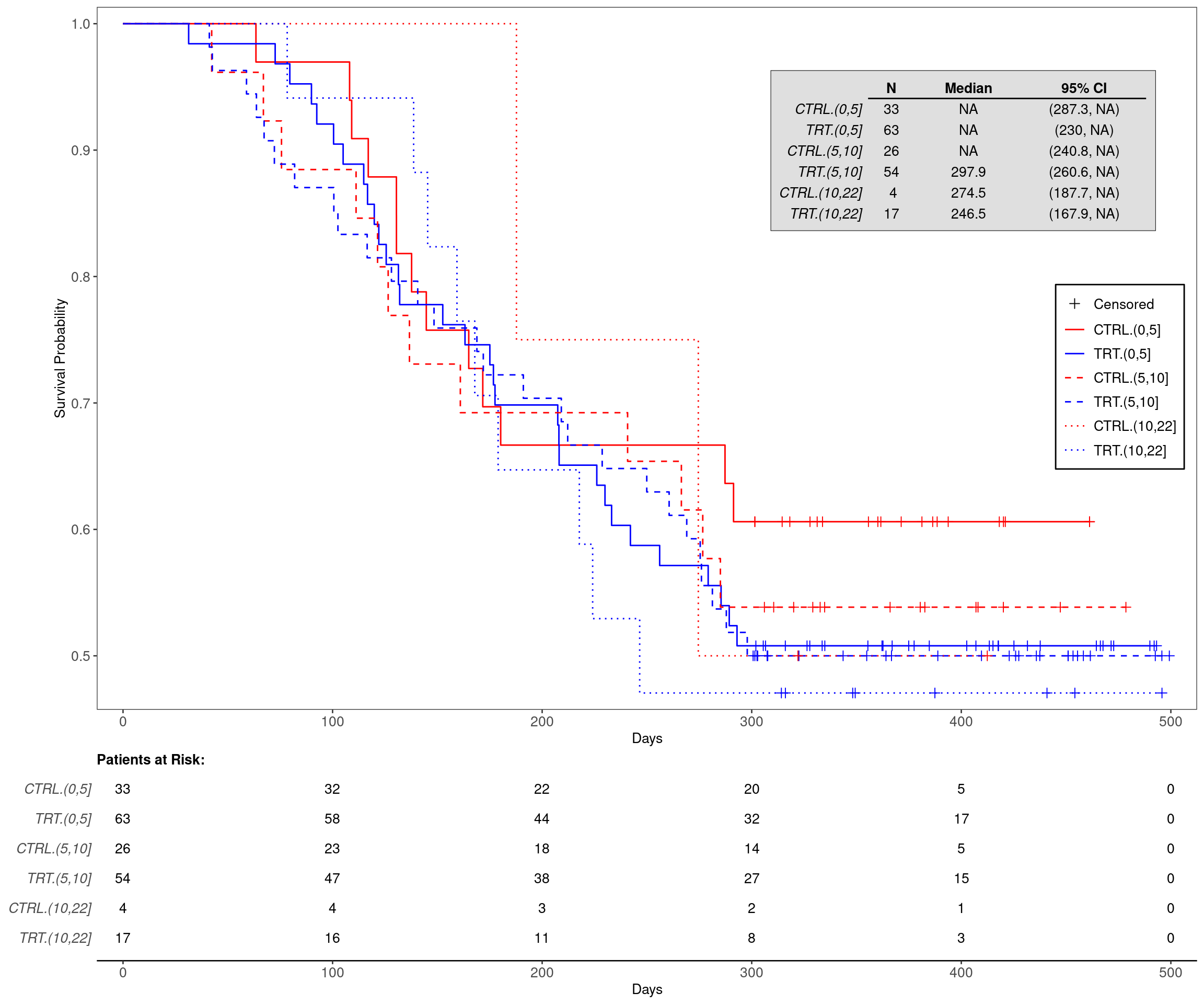
The advantage of using the cut() function is that it is sufficient to add additional cutoffs in order to obtain more than two bins for the cut version of the continuous biomarker variable. Again we can check the order of the factor levels to determine the col and lty arguments for g_km(). Here we want to always use red for the control and blue for the treatment arm, and then vary the line type for the different biomarker bins.

Code

adtte3 <- adtte %>%
  mutate(
    BMRKR1_CAT = cut(BMRKR1, c(0, 5, 10, 22)),
    ARM_BMRKR1 = interaction(ARM_BIN, BMRKR1_CAT)
  )
levels(adtte3$ARM_BMRKR1)

[1] "CTRL.(0,5]"   "TRT.(0,5]"    "CTRL.(5,10]"  "TRT.(5,10]"   "CTRL.(10,22]"
[6] "TRT.(10,22]"

Code

g_km(
  df = adtte3,
  variables = variables,
  annot_surv_med = TRUE,
  col = c("red", "blue", "red", "blue", "red", "blue"),
  lty = c(1, 1, 2, 2, 3, 3)
)

Code

sessionInfo()

R version 4.4.2 (2024-10-31)
Platform: x86_64-pc-linux-gnu
Running under: Ubuntu 24.04.1 LTS

Matrix products: default
BLAS:   /usr/lib/x86_64-linux-gnu/openblas-pthread/libblas.so.3 
LAPACK: /usr/lib/x86_64-linux-gnu/openblas-pthread/libopenblasp-r0.3.26.so;  LAPACK version 3.12.0

locale:
 [1] LC_CTYPE=en_US.UTF-8       LC_NUMERIC=C              
 [3] LC_TIME=en_US.UTF-8        LC_COLLATE=en_US.UTF-8    
 [5] LC_MONETARY=en_US.UTF-8    LC_MESSAGES=en_US.UTF-8   
 [7] LC_PAPER=en_US.UTF-8       LC_NAME=C                 
 [9] LC_ADDRESS=C               LC_TELEPHONE=C            
[11] LC_MEASUREMENT=en_US.UTF-8 LC_IDENTIFICATION=C       

time zone: Etc/UTC
tzcode source: system (glibc)

attached base packages:
[1] stats     graphics  grDevices utils     datasets  methods   base     

other attached packages:
[1] dplyr_1.1.4       tern_0.9.7        rtables_0.6.11    magrittr_2.0.3   
[5] formatters_0.5.10

loaded via a namespace (and not attached):
 [1] Matrix_1.7-2             gtable_0.3.6             jsonlite_1.9.0          
 [4] compiler_4.4.2           tidyselect_1.2.1         stringr_1.5.1           
 [7] tidyr_1.3.1              splines_4.4.2            scales_1.3.0            
[10] yaml_2.3.10              fastmap_1.2.0            lattice_0.22-6          
[13] ggplot2_3.5.1            R6_2.6.1                 labeling_0.4.3          
[16] generics_0.1.3           knitr_1.49               forcats_1.0.0           
[19] rbibutils_2.3            htmlwidgets_1.6.4        backports_1.5.0         
[22] checkmate_2.3.2          tibble_3.2.1             munsell_0.5.1           
[25] pillar_1.10.1            rlang_1.1.5              broom_1.0.7             
[28] stringi_1.8.4            xfun_0.51                cli_3.6.4               
[31] withr_3.0.2              Rdpack_2.6.2             digest_0.6.37           
[34] grid_4.4.2               cowplot_1.1.3            lifecycle_1.0.4         
[37] vctrs_0.6.5              evaluate_1.0.3           glue_1.8.0              
[40] farver_2.1.2             nestcolor_0.1.3          codetools_0.2-20        
[43] survival_3.8-3           random.cdisc.data_0.3.16 colorspace_2.1-1        
[46] rmarkdown_2.29           purrr_1.0.4              tools_4.4.2             
[49] pkgconfig_2.0.3          htmltools_0.5.8.1

Reuse