Visit All Patients
Statistics (N=400)
———————————————————————————————————————
WEEK 1 DAY 8
n 400
Adjusted Mean (SE) 3.615 (0.620)
95% CI (2.396, 4.834)
WEEK 2 DAY 15
n 400
Adjusted Mean (SE) 8.870 (0.602)
95% CI (7.687, 10.053)
WEEK 3 DAY 22
n 400
Adjusted Mean (SE) 15.094 (0.683)
95% CI (13.751, 16.437)
WEEK 4 DAY 29
n 400
Adjusted Mean (SE) 19.009 (0.717)
95% CI (17.599, 20.418)
WEEK 5 DAY 36
n 400
Adjusted Mean (SE) 24.028 (0.747)
95% CI (22.560, 25.496)
Adding baseline rows
It may be of interest to summarize some different statistics at the baseline visit or summarize a different variable in the data set not used in the MMRM. For example, the model may use the variable CHG but the baseline visit row may summarize the AVAL variable, thus we would need to create two tables and then combine them to accomplish this.
Code
# First have the least-square means table.a <-basic_table(show_colcounts =TRUE) %>%split_cols_by("ARMCD", ref_group = mmrm_results$ref_level) %>%split_rows_by("AVISIT", split_fun = split_fun, label_pos ="topleft", split_label =obj_label(df$AVISIT)) %>%summarize_lsmeans(show_relative ="increase") %>%append_topleft(" Statistics") %>%build_table(df, alt_counts_df = adsl_sub)# Second prepare the baseline values summary table.baseline_dat <- adqs %>%filter(AVISIT =="BASELINE") %>%distinct(USUBJID, .keep_all =TRUE) %>%droplevels()b <-basic_table(show_colcounts =TRUE) %>%split_cols_by("ARMCD") %>%split_rows_by("AVISIT") %>%analyze_vars("AVAL") %>%append_topleft(" Statistics") %>%build_table(baseline_dat, alt_counts_df = adsl_sub)# Now we can combine them as follows.col_info(b) <- EmptyColInforbind(b, a)
Visit ARM B ARM A ARM C
Statistics (N=134) (N=134) (N=132)
————————————————————————————————————————————————————————————————————————————————————————————
BASELINE
n 134 134 132
Mean (SD) 49.9 (7.4) 49.7 (8.3) 50.3 (9.1)
Median 48.7 49.3 49.7
Min - Max 33.7 - 65.9 25.8 - 71.5 26.0 - 70.0
WEEK 1 DAY 8
n 134 134 132
Adjusted Mean (SE) 3.488 (0.687) 4.246 (0.687) 3.163 (0.692)
95% CI (2.136, 4.839) (2.895, 5.598) (1.803, 4.523)
Difference in Adjusted Means (SE) 0.759 (0.973) -0.325 (0.976)
95% CI (-1.155, 2.672) (-2.243, 1.593)
Relative Increase (%) 21.8% -9.3%
p-value (MMRM) 0.4362 0.7393
WEEK 2 DAY 15
n 134 134 132
Adjusted Mean (SE) 9.135 (0.768) 9.018 (0.767) 8.509 (0.773)
95% CI (7.626, 10.644) (7.510, 10.527) (6.991, 10.028)
Difference in Adjusted Means (SE) -0.117 (1.087) -0.626 (1.090)
95% CI (-2.253, 2.020) (-2.768, 1.517)
Relative Increase (%) -1.3% -6.8%
p-value (MMRM) 0.9147 0.5662
WEEK 3 DAY 22
n 134 134 132
Adjusted Mean (SE) 13.547 (0.871) 16.014 (0.871) 15.789 (0.877)
95% CI (11.835, 15.259) (14.303, 17.726) (14.066, 17.513)
Difference in Adjusted Means (SE) 2.467 (1.232) 2.242 (1.236)
95% CI (0.044, 4.890) (-0.187, 4.672)
Relative Increase (%) 18.2% 16.6%
p-value (MMRM) 0.0460 0.0704
WEEK 4 DAY 29
n 134 134 132
Adjusted Mean (SE) 18.102 (0.995) 19.479 (0.995) 19.511 (1.002)
95% CI (16.146, 20.059) (17.523, 21.435) (17.541, 21.481)
Difference in Adjusted Means (SE) 1.377 (1.408) 1.409 (1.413)
95% CI (-1.392, 4.145) (-1.368, 4.186)
Relative Increase (%) 7.6% 7.8%
p-value (MMRM) 0.3288 0.3192
WEEK 5 DAY 36
n 134 134 132
Adjusted Mean (SE) 23.503 (1.058) 24.931 (1.058) 23.704 (1.065)
95% CI (21.423, 25.583) (22.851, 27.011) (21.610, 25.798)
Difference in Adjusted Means (SE) 1.428 (1.497) 0.201 (1.502)
95% CI (-1.515, 4.371) (-2.752, 3.153)
Relative Increase (%) 6.1% 0.9%
p-value (MMRM) 0.3408 0.8937
Considering visit averages
It may also be of interest to summarize several different statistics for an averaged combination of various visits in the MMRM. For example, you may want to see the statistics for the average of the first 2 visits, or the average statistics of all visits combined. This can be accomplished by specifying the averages_emmeans argument when fitting the MMRM model.
Code
mmrm_results_avg_visits <-fit_mmrm(vars =list(response ="CHG",covariates =c("BASE", "STRATA1", "BMRKR2"),id ="USUBJID",arm ="ARMCD",visit ="AVISIT" ),data = adqs_f,weights_emmeans ="equal",averages_emmeans =list("WEEKS 1-2"=c("WEEK 1 DAY 8", "WEEK 2 DAY 15"),"WEEKS 3-5"=c("WEEK 3 DAY 22", "WEEK 4 DAY 29", "WEEK 5 DAY 36"),"ALL VISITS"=c("WEEK 1 DAY 8", "WEEK 2 DAY 15", "WEEK 3 DAY 22", "WEEK 4 DAY 29", "WEEK 5 DAY 36") ))df_avgs <-tidy(mmrm_results_avg_visits)attr(df_avgs$AVISIT, "label") <-"Visit"# Define the split functionsplit_fun <- drop_split_levelsresult <-basic_table(show_colcounts =TRUE) %>%split_cols_by("ARMCD", ref_group = mmrm_results_avg_visits$ref_level) %>%split_rows_by("AVISIT", split_fun = split_fun, label_pos ="topleft", split_label =obj_label(df_avgs$AVISIT)) %>%summarize_lsmeans(show_relative ="increase") %>%append_topleft(" Statistics") %>%build_table(df_avgs, alt_counts_df = adsl_sub)result
Visit ARM B ARM A ARM C
Statistics (N=134) (N=134) (N=132)
————————————————————————————————————————————————————————————————————————————————————————————
WEEK 1 DAY 8
n 134 134 132
Adjusted Mean (SE) 3.488 (0.687) 4.246 (0.687) 3.163 (0.692)
95% CI (2.136, 4.839) (2.895, 5.598) (1.803, 4.523)
Difference in Adjusted Means (SE) 0.759 (0.973) -0.325 (0.976)
95% CI (-1.155, 2.672) (-2.243, 1.593)
Relative Increase (%) 21.8% -9.3%
p-value (MMRM) 0.4362 0.7393
WEEK 2 DAY 15
n 134 134 132
Adjusted Mean (SE) 9.135 (0.768) 9.018 (0.767) 8.509 (0.773)
95% CI (7.626, 10.644) (7.510, 10.527) (6.991, 10.028)
Difference in Adjusted Means (SE) -0.117 (1.087) -0.626 (1.090)
95% CI (-2.253, 2.020) (-2.768, 1.517)
Relative Increase (%) -1.3% -6.8%
p-value (MMRM) 0.9147 0.5662
WEEK 3 DAY 22
n 134 134 132
Adjusted Mean (SE) 13.547 (0.871) 16.014 (0.871) 15.789 (0.877)
95% CI (11.835, 15.259) (14.303, 17.726) (14.066, 17.513)
Difference in Adjusted Means (SE) 2.467 (1.232) 2.242 (1.236)
95% CI (0.044, 4.890) (-0.187, 4.672)
Relative Increase (%) 18.2% 16.6%
p-value (MMRM) 0.0460 0.0704
WEEK 4 DAY 29
n 134 134 132
Adjusted Mean (SE) 18.102 (0.995) 19.479 (0.995) 19.511 (1.002)
95% CI (16.146, 20.059) (17.523, 21.435) (17.541, 21.481)
Difference in Adjusted Means (SE) 1.377 (1.408) 1.409 (1.413)
95% CI (-1.392, 4.145) (-1.368, 4.186)
Relative Increase (%) 7.6% 7.8%
p-value (MMRM) 0.3288 0.3192
WEEK 5 DAY 36
n 134 134 132
Adjusted Mean (SE) 23.503 (1.058) 24.931 (1.058) 23.704 (1.065)
95% CI (21.423, 25.583) (22.851, 27.011) (21.610, 25.798)
Difference in Adjusted Means (SE) 1.428 (1.497) 0.201 (1.502)
95% CI (-1.515, 4.371) (-2.752, 3.153)
Relative Increase (%) 6.1% 0.9%
p-value (MMRM) 0.3408 0.8937
WEEKS 1-2
n 134 134 132
Adjusted Mean (SE) 6.311 (0.514) 6.632 (0.514) 5.836 (0.516)
95% CI (5.301, 7.322) (5.623, 7.642) (4.821, 6.852)
Difference in Adjusted Means (SE) 0.321 (0.728) -0.475 (0.729)
95% CI (-1.111, 1.753) (-1.909, 0.959)
Relative Increase (%) 5.1% -7.5%
p-value (MMRM) 0.6596 0.5151
WEEKS 3-5
n 134 134 132
Adjusted Mean (SE) 18.384 (0.560) 20.141 (0.560) 19.668 (0.563)
95% CI (17.284, 19.485) (19.041, 21.241) (18.562, 20.775)
Difference in Adjusted Means (SE) 1.757 (0.793) 1.284 (0.794)
95% CI (0.198, 3.316) (-0.278, 2.846)
Relative Increase (%) 9.6% 7.0%
p-value (MMRM) 0.0273 0.1068
ALL VISITS
n 134 134 132
Adjusted Mean (SE) 13.555 (0.388) 14.738 (0.388) 14.135 (0.389)
95% CI (12.792, 14.318) (13.976, 15.500) (13.370, 14.900)
Difference in Adjusted Means (SE) 1.183 (0.551) 0.580 (0.551)
95% CI (0.100, 2.266) (-0.502, 1.663)
Relative Increase (%) 8.7% 4.3%
p-value (MMRM) 0.0324 0.2924
WEEK 1 DAY 8 WEEK 2 DAY 15 WEEK 3 DAY 22 WEEK 4 DAY 29 WEEK 5 DAY 36
————————————————————————————————————————————————————————————————————————————————————————————
WEEK 1 DAY 8 63.0140 -0.6664 2.5965 -1.6231 0.2589
WEEK 2 DAY 15 -0.6664 78.6592 1.7004 -11.8677 -0.4261
WEEK 3 DAY 22 2.5965 1.7004 101.2949 -5.8424 7.1145
WEEK 4 DAY 29 -1.6231 -11.8677 -5.8424 132.4034 -5.3739
WEEK 5 DAY 36 0.2589 -0.4261 7.1145 -5.3739 149.6937
Model diagnostics are currently available to evaluate choice of covariates for the fixed and random effects. Statistics to evaluate choice of covariance structure are being investigated and will be included in a future release.
library(dplyr)library(tern.mmrm)library(broom)adsl <- random.cdisc.data::cadsladqs <- random.cdisc.data::cadqs# Ensure character variables are converted to factors and empty strings and NAs are explicit missing levels.adsl <-df_explicit_na(adsl)adqs <-df_explicit_na(adqs)adqs_f <- adqs %>% dplyr::filter(PARAMCD =="FKSI-FWB"&!AVISIT %in%c("BASELINE", "SCREENING")) %>%droplevels() %>% dplyr::mutate(ARMCD =factor(ARMCD, levels =c("ARM B", "ARM A", "ARM C"))) %>% dplyr::mutate(AVISITN =rank(AVISITN) %>%as.factor() %>%as.numeric() %>%as.factor() )adsl_sub <- adqs_f %>% dplyr::filter(!is.na(CHG)) %>%distinct(USUBJID) %>%left_join(adsl, by ="USUBJID")var_labels(adqs_f) <-var_labels(adqs)
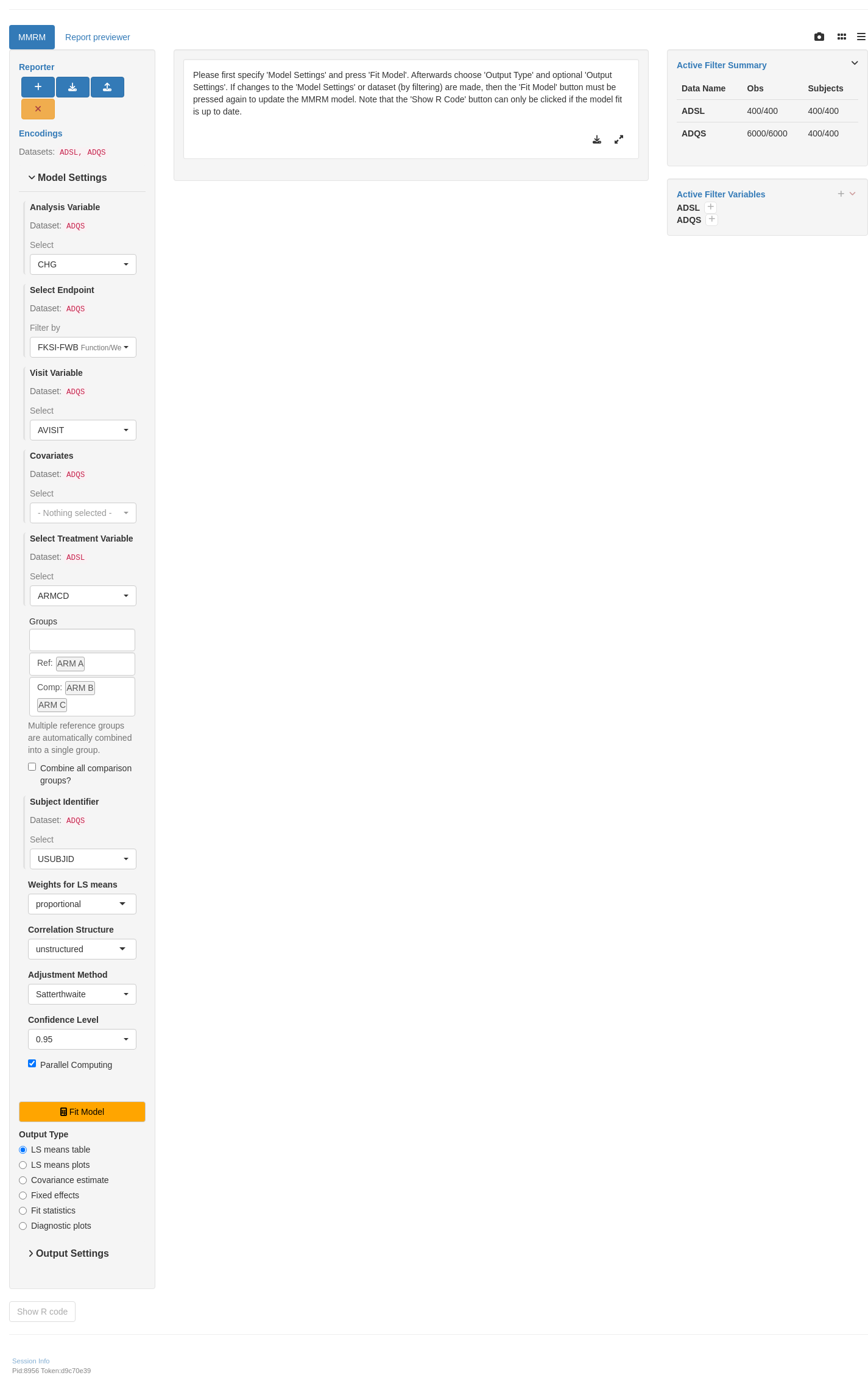
teal App
Code
library(teal.modules.clinical)## Data reproducible codedata <-teal_data()data <-within(data, {library(dplyr) ADSL <- random.cdisc.data::cadsl ADQS <- random.cdisc.data::cadqs %>%filter(ABLFL !="Y"& ABLFL2 !="Y") %>%filter(AVISIT %in%c("WEEK 1 DAY 8", "WEEK 2 DAY 15", "WEEK 3 DAY 22")) %>%mutate(AVISIT =as.factor(AVISIT),AVISITN =rank(AVISITN) %>%as.factor() %>%as.numeric() %>%as.factor() # making consecutive numeric factor )})datanames <-c("ADSL", "ADQS")datanames(data) <- datanames
Warning: `datanames<-()` was deprecated in teal.data 0.6.1.
ℹ invalid to use `datanames()<-` or `names()<-` on an object of class
`teal_data`. See ?names.teal_data
---title: MMRMT01subtitle: Tables for Mixed-Effect Model Repeated Measures Analysis---------------------------------------------------------------------------{{< include ../../_utils/envir_hook.qmd >}}```{r setup, echo = FALSE, warning = FALSE, message = FALSE}library(dplyr)library(tern.mmrm)library(broom)adsl <- random.cdisc.data::cadsladqs <- random.cdisc.data::cadqs# Ensure character variables are converted to factors and empty strings and NAs are explicit missing levels.adsl <- df_explicit_na(adsl)adqs <- df_explicit_na(adqs)adqs_f <- adqs %>% dplyr::filter(PARAMCD == "FKSI-FWB" & !AVISIT %in% c("BASELINE", "SCREENING")) %>% droplevels() %>% dplyr::mutate(ARMCD = factor(ARMCD, levels = c("ARM B", "ARM A", "ARM C"))) %>% dplyr::mutate( AVISITN = rank(AVISITN) %>% as.factor() %>% as.numeric() %>% as.factor() )adsl_sub <- adqs_f %>% dplyr::filter(!is.na(CHG)) %>% distinct(USUBJID) %>% left_join(adsl, by = "USUBJID")var_labels(adqs_f) <- var_labels(adqs)```::: panel-tabset## Least Squares Means#### Considering the treatment variable in the model```{r variant1, test = list(result_v1 = "result"), message = FALSE}mmrm_results <- fit_mmrm( vars = list( response = "CHG", covariates = c("BASE", "STRATA1", "BMRKR2"), id = "USUBJID", arm = "ARMCD", visit = "AVISIT" ), data = adqs_f, weights_emmeans = "equal")df <- tidy(mmrm_results)attr(df$AVISIT, "label") <- "Visit"# Define the split functionsplit_fun <- drop_split_levelsresult <- basic_table(show_colcounts = TRUE) %>% split_cols_by("ARMCD", ref_group = mmrm_results$ref_level) %>% split_rows_by("AVISIT", split_fun = split_fun, label_pos = "topleft", split_label = obj_label(df$AVISIT)) %>% summarize_lsmeans(show_relative = "increase") %>% append_topleft(" Statistics") %>% build_table(df, alt_counts_df = adsl_sub)result```#### Not considering the treatment variable in the model```{r variant2, test = list(result_v2 = "result")}mmrm_results_no_arm <- fit_mmrm( vars = list( response = "CHG", covariates = c("BMRKR2", "STRATA1"), id = "USUBJID", visit = "AVISIT" ), data = adqs_f, weights_emmeans = "equal", parallel = TRUE)df_no_arm <- tidy(mmrm_results_no_arm)attr(df_no_arm$AVISIT, "label") <- "Visit"# Define the split functionsplit_fun <- drop_split_levelsresult <- basic_table(show_colcounts = TRUE) %>% add_overall_col("All Patients") %>% split_rows_by("AVISIT", split_fun = split_fun, label_pos = "topleft", split_label = obj_label(df_no_arm$AVISIT)) %>% summarize_lsmeans(arms = FALSE) %>% append_topleft(" Statistics") %>% build_table(df_no_arm, alt_counts_df = adsl_sub)result```#### Adding baseline rowsIt may be of interest to summarize some different statistics at the baseline visit or summarize a different variable in the data set not used in the MMRM. For example, the model may use the variable `CHG` but the baseline visit row may summarize the `AVAL` variable, thus we would need to create two tables and then combine them to accomplish this.```{r variant_baseline, test = list(result_baseline = "result")}# First have the least-square means table.a <- basic_table(show_colcounts = TRUE) %>% split_cols_by("ARMCD", ref_group = mmrm_results$ref_level) %>% split_rows_by("AVISIT", split_fun = split_fun, label_pos = "topleft", split_label = obj_label(df$AVISIT)) %>% summarize_lsmeans(show_relative = "increase") %>% append_topleft(" Statistics") %>% build_table(df, alt_counts_df = adsl_sub)# Second prepare the baseline values summary table.baseline_dat <- adqs %>% filter(AVISIT == "BASELINE") %>% distinct(USUBJID, .keep_all = TRUE) %>% droplevels()b <- basic_table(show_colcounts = TRUE) %>% split_cols_by("ARMCD") %>% split_rows_by("AVISIT") %>% analyze_vars("AVAL") %>% append_topleft(" Statistics") %>% build_table(baseline_dat, alt_counts_df = adsl_sub)# Now we can combine them as follows.col_info(b) <- EmptyColInforbind(b, a)```#### Considering visit averagesIt may also be of interest to summarize several different statistics for an averaged combination of various visits in the MMRM. For example, you may want to see the statistics for the average of the first 2 visits, or the average statistics of all visits combined. This can be accomplished by specifying the `averages_emmeans` argument when fitting the MMRM model.```{r variant3, test = list(result_v3 = "result")}mmrm_results_avg_visits <- fit_mmrm( vars = list( response = "CHG", covariates = c("BASE", "STRATA1", "BMRKR2"), id = "USUBJID", arm = "ARMCD", visit = "AVISIT" ), data = adqs_f, weights_emmeans = "equal", averages_emmeans = list( "WEEKS 1-2" = c("WEEK 1 DAY 8", "WEEK 2 DAY 15"), "WEEKS 3-5" = c("WEEK 3 DAY 22", "WEEK 4 DAY 29", "WEEK 5 DAY 36"), "ALL VISITS" = c("WEEK 1 DAY 8", "WEEK 2 DAY 15", "WEEK 3 DAY 22", "WEEK 4 DAY 29", "WEEK 5 DAY 36") ))df_avgs <- tidy(mmrm_results_avg_visits)attr(df_avgs$AVISIT, "label") <- "Visit"# Define the split functionsplit_fun <- drop_split_levelsresult <- basic_table(show_colcounts = TRUE) %>% split_cols_by("ARMCD", ref_group = mmrm_results_avg_visits$ref_level) %>% split_rows_by("AVISIT", split_fun = split_fun, label_pos = "topleft", split_label = obj_label(df_avgs$AVISIT)) %>% summarize_lsmeans(show_relative = "increase") %>% append_topleft(" Statistics") %>% build_table(df_avgs, alt_counts_df = adsl_sub)result```## Fixed Effects#### Considering the treatment variable in the model```{r}as.rtable(mmrm_results, type ="fixed")```#### Not considering the treatment variable in the model```{r}as.rtable(mmrm_results_no_arm, type ="fixed")```## Covariance Matrix```{r}as.rtable(mmrm_results, type ="cov")```## Model DiagnosticsModel diagnostics are currently available to evaluate choice of covariates for the fixed and random effects. Statistics to evaluate choice of covariance structure are being investigated and will be included in a future release.```{r}as.rtable(mmrm_results, type ="diagnostic")```## Data Setup```{r setup}#| code-fold: show```:::{{< include ../../_utils/save_results.qmd >}}## `teal` App```{r teal, opts.label = c("skip_if_testing", "app")}library(teal.modules.clinical)## Data reproducible codedata <- teal_data()data <- within(data, { library(dplyr) ADSL <- random.cdisc.data::cadsl ADQS <- random.cdisc.data::cadqs %>% filter(ABLFL != "Y" & ABLFL2 != "Y") %>% filter(AVISIT %in% c("WEEK 1 DAY 8", "WEEK 2 DAY 15", "WEEK 3 DAY 22")) %>% mutate( AVISIT = as.factor(AVISIT), AVISITN = rank(AVISITN) %>% as.factor() %>% as.numeric() %>% as.factor() # making consecutive numeric factor )})datanames <- c("ADSL", "ADQS")datanames(data) <- datanamesjoin_keys(data) <- default_cdisc_join_keys[datanames]## Reusable Configuration For ModulesADQS <- data[["ADQS"]]arm_ref_comp <- list( ARMCD = list( ref = "ARM A", comp = c("ARM B", "ARM C") ))## Setup Appapp <- init( data = data, modules = modules( tm_a_mmrm( label = "MMRM", dataname = "ADQS", aval_var = choices_selected(c("AVAL", "CHG"), "CHG"), id_var = choices_selected(c("USUBJID", "SUBJID"), "USUBJID"), arm_var = choices_selected(c("ARM", "ARMCD"), "ARMCD"), visit_var = choices_selected(c("AVISIT", "AVISITN"), "AVISIT"), arm_ref_comp = arm_ref_comp, paramcd = choices_selected( choices = value_choices(ADQS, "PARAMCD", "PARAM"), selected = "FKSI-FWB" ), cov_var = choices_selected(c("BASE", "AGE", "SEX", "BASE:AVISIT"), NULL), conf_level = choices_selected(c(0.95, 0.9, 0.8), 0.95) ) ))shinyApp(app$ui, app$server)```{{< include ../../repro.qmd >}}