---
title: COXT01
subtitle: Cox Regression
---
------------------------------------------------------------------------
{{< include ../../_utils/envir_hook.qmd >}}
```{r setup, echo = FALSE, warning = FALSE, message = FALSE}
library(dplyr)
library(tern)
adsl <- random.cdisc.data::cadsl
adtte <- random.cdisc.data::cadtte
# Ensure character variables are converted to factors and empty strings and NAs are explicit missing levels.
adsl <- df_explicit_na(adsl)
adtte <- df_explicit_na(adtte)
adsl_filtered <- adsl %>% dplyr::filter(
RACE %in% c("ASIAN", "BLACK OR AFRICAN AMERICAN", "WHITE")
)
adtte_filtered <- dplyr::inner_join(
x = adsl_filtered[, c("STUDYID", "USUBJID")],
y = adtte,
by = c("STUDYID", "USUBJID")
)
anl <- adtte_filtered %>%
filter(PARAMCD == "OS") %>%
mutate(EVENT = 1 - CNSR) %>%
filter(ARM %in% c("B: Placebo", "A: Drug X")) %>%
mutate(ARM = droplevels(relevel(ARM, "B: Placebo"))) %>%
mutate(RACE = droplevels(RACE) %>% formatters::with_label("Race"))
# Add variable for column split label
anl <- anl %>% mutate(col_label = "Treatment Effect Adjusted for Covariate")
```
```{r include = FALSE}
webr_code_labels <- c("setup")
```
{{< include ../../_utils/webr_no_include.qmd >}}
## Output
Cox models are the most commonly used methods to estimate the magnitude of the effect in survival analyses. It assumes proportional hazards; that is, it assumes that the ratio of the hazards of the two groups (e.g. two arms) is constant over time. This ratio is referred to as the "hazard ratio" and is one of the most commonly reported metrics to describe the effect size in survival analysis.
::::::: panel-tabset
## Cox Regression
The `summarize_coxreg` function fits, tidies and arranges a Cox regression model in a table layout using the `rtables` framework. For a Cox regression model, arguments `variables`, `control`, and `at` can be specified (see `?summarize_coxreg` for more details and customization options). All variables specified within `variables` must be present in the data used when building the table.
To see the same model as a `data.frame` object, these three arguments (as well as the data) can be passed to the `fit_coxreg_univar` function, and the resulting list tidied using `broom::tidy()`.
::: {.panel-tabset .nav-justified group="webr"}
## {{< fa regular file-lines sm fw >}} Preview
```{r variant1, test = list(result_v1 = "result")}
variables <- list(
  time = "AVAL",
  event = "EVENT",
  arm = "ARM",
  covariates = c("AGE", "SEX", "RACE")
)

lyt <- basic_table() %>%
  split_cols_by("col_label") %>%
  summarize_coxreg(variables = variables) %>%
  append_topleft("Effect/Covariate Included in the Model")

result <- build_table(lyt = lyt, df = anl)
result
```
```{r include = FALSE}
webr_code_labels <- c("variant1")
```
{{< include ../../_utils/webr.qmd >}}
:::
## Cox Regression <br/> with Interaction Term
The argument `control` can be used to modify standard outputs; `control_coxreg()` helps in adopting the right settings (see `?control_coxreg`). For instance, `control` is used to include the interaction terms.
::: {.panel-tabset .nav-justified group="webr"}
## {{< fa regular file-lines sm fw >}} Preview
```{r variant2, test = list(result_v2 = "result")}
variables <- list(
  time = "AVAL",
  event = "EVENT",
  arm = "ARM",
  covariates = c("AGE", "RACE")
)

lyt <- basic_table() %>%
  split_cols_by("col_label") %>%
  summarize_coxreg(
    variables = variables,
    control = control_coxreg(interaction = TRUE),
    .stats = c("n", "hr", "ci", "pval", "pval_inter")
  ) %>%
  append_topleft("Effect/Covariate Included in the Model")

result <- build_table(lyt = lyt, df = anl)
result
```
```{r include = FALSE}
webr_code_labels <- c("variant2")
```
{{< include ../../_utils/webr.qmd >}}
:::
## Cox Regression <br/> Specifying Covariates
The optional argument `at` allows the user to provide the expected level of estimation for the interaction when the predictor is a quantitative variable. For instance, it might be relevant to choose the age at which the hazard ratio should be estimated. If no input is provided to `at`, the median value is used in the row name (as in the previous tab).
::: {.panel-tabset .nav-justified group="webr"}
## {{< fa regular file-lines sm fw >}} Preview
```{r variant3, test = list(result_v3 = "result")}
variables <- list(
  time = "AVAL",
  event = "EVENT",
  arm = "ARM",
  covariates = c("AGE", "SEX")
)

lyt <- basic_table() %>%
  split_cols_by("col_label") %>%
  summarize_coxreg(
    variables = variables,
    control = control_coxreg(interaction = TRUE),
    at = list(AGE = c(30, 40, 50)),
    .stats = c("n", "hr", "ci", "pval", "pval_inter")
  ) %>%
  append_topleft("Effect/Covariate Included in the Model")

result <- build_table(lyt = lyt, df = anl)
result
```
```{r include = FALSE}
webr_code_labels <- c("variant3")
```
{{< include ../../_utils/webr.qmd >}}
:::
## Cox Regression Setting <br/> Strata, Ties, Alpha Level
Additional controls can be customized using `control_coxreg` (see `?control_coxreg`) such as the ties calculation method and the confidence level. Stratification variables can be added via the `strata` element of the `variables` list.
::: {.panel-tabset .nav-justified group="webr"}
## {{< fa regular file-lines sm fw >}} Preview
```{r variant4, test = list(result_v4 = "result")}
variables <- list(
  time = "AVAL",
  event = "EVENT",
  arm = "ARM",
  covariates = c("AGE", "RACE"),
  strata = "SEX"
)

control <- control_coxreg(
  ties = "breslow",
  interaction = TRUE,
  conf_level = 0.90
)

lyt <- basic_table() %>%
  split_cols_by("col_label") %>%
  summarize_coxreg(
    variables = variables,
    control = control,
    at = list(AGE = c(30, 40, 50)),
    .stats = c("n", "hr", "ci", "pval", "pval_inter")
  ) %>%
  append_topleft("Effect/Covariate Included in the Model")

result <- build_table(lyt = lyt, df = anl)
result
```
```{r include = FALSE}
webr_code_labels <- c("variant4")
```
{{< include ../../_utils/webr.qmd >}}
:::
## Data Setup
```{r setup}
#| code-fold: show
```
:::::::
{{< include ../../_utils/save_results.qmd >}}
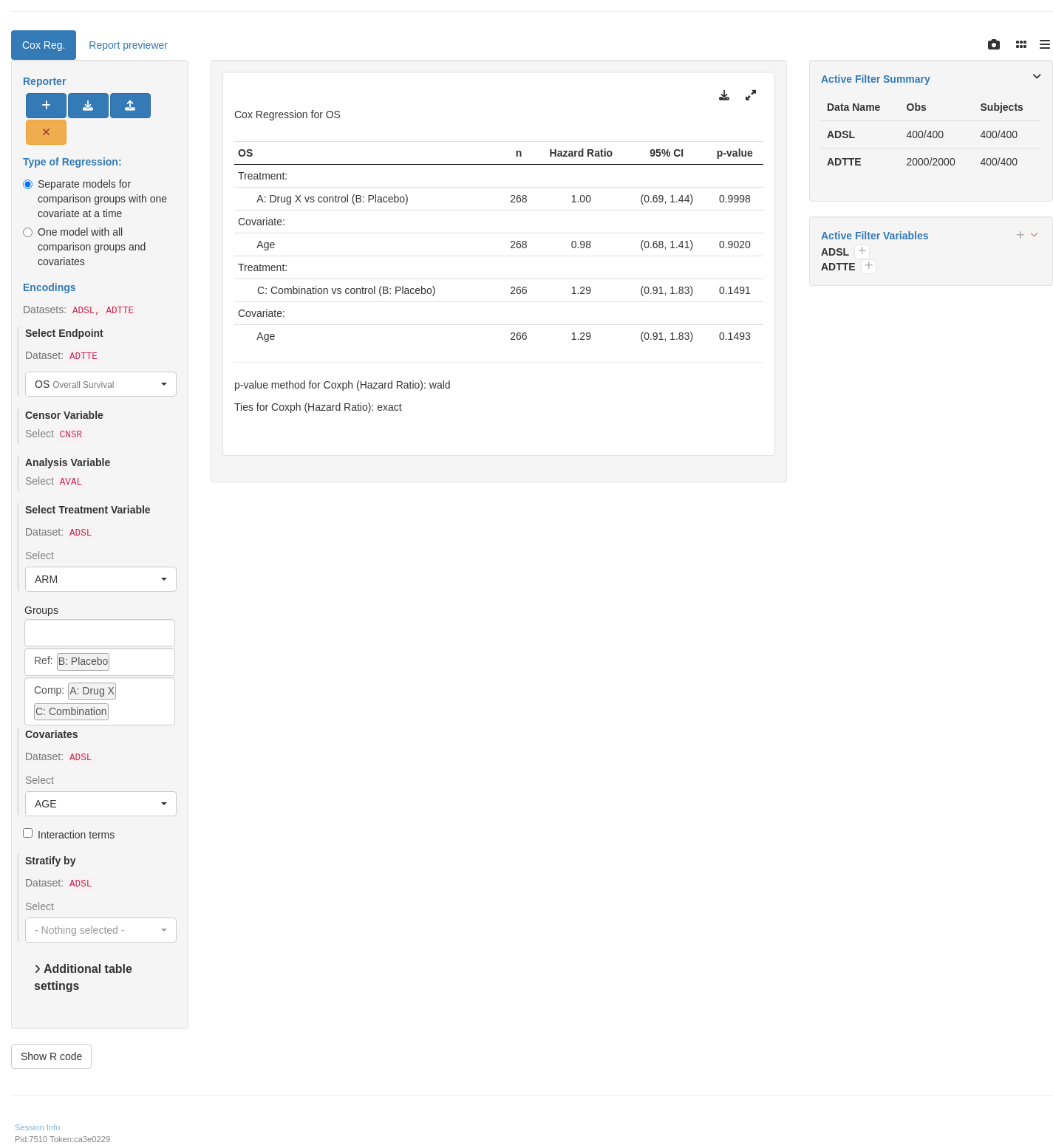
## `teal` App
::: {.panel-tabset .nav-justified}
## {{< fa regular file-lines fa-sm fa-fw >}} Preview
```{r teal, opts.label = c("skip_if_testing", "app")}
library(teal.modules.clinical)

arm_ref_comp <- list(
  ACTARMCD = list(
    ref = "ARM B",
    comp = c("ARM A", "ARM C")
  ),
  ARM = list(
    ref = "B: Placebo",
    comp = c("A: Drug X", "C: Combination")
  )
)

## Data reproducible code
data <- teal_data()
data <- within(data, {
  ADSL <- random.cdisc.data::cadsl
  ADTTE <- random.cdisc.data::cadtte

  # Ensure character variables are converted to factors and empty strings and NAs are explicit missing levels.
  ADSL <- df_explicit_na(ADSL)
  ADTTE <- df_explicit_na(ADTTE)
})
join_keys(data) <- default_cdisc_join_keys[c("ADSL", "ADTTE")]

## Reusable Configuration For Modules
ADTTE <- data[["ADTTE"]]

## Setup App
app <- init(
  data = data,
  modules = modules(
    tm_t_coxreg(
      label = "Cox Reg.",
      dataname = "ADTTE",
      arm_var = choices_selected(c("ARM", "ACTARMCD"), "ARM"),
      arm_ref_comp = arm_ref_comp,
      paramcd = choices_selected(
        value_choices(ADTTE, "PARAMCD", "PARAM"), "OS"
      ),
      strata_var = choices_selected(
        c("SEX", "STRATA1", "STRATA2"), NULL
      ),
      cov_var = choices_selected(
        c("AGE", "SEX", "RACE"), "AGE"
      ),
      multivariate = FALSE
    )
  )
)
shinyApp(app$ui, app$server)
```
{{< include ../../_utils/shinylive.qmd >}}
:::
{{< include ../../repro.qmd >}}

