SPG1

STEP Graphs for Survival Outcome

SPG

We will use the cadtte data set from the random.cdisc.data package to create the STEP survival graph. We start by filtering the adtte data set for the overall survival observations, converting time of overall survival to months, creating a new variable for event information, binarizing the ARM variable, and discarding BMRKR1 values for the non-BEP. We also relabel the biomarker evaluable population flag variable BEP01FL.

Code

library(tern)
library(ggplot2.utils)
library(dplyr)

adtte <- random.cdisc.data::cadtte %>%
  df_explicit_na() %>%
  filter(
    PARAMCD == "OS"
  ) %>%
  mutate(
    AVAL = day2month(AVAL),
    AVALU = "Months",
    is_event = CNSR == 0,
    ARM_BIN = fct_collapse_only(
      ARM,
      CTRL = c("B: Placebo"),
      TRT = c("A: Drug X", "C: Combination")
    ),
    BMRKR1 = ifelse(BEP01FL == "N", NA, BMRKR1)
  ) %>%
  var_relabel(
    BEP01FL = "BEP"
  )

We then perform with the fit_survival_step() function the required calculations: this function fits the Subgroup Treatment Effect Pattern (STEP) models for the survival outcome within each of the percentile intervals of the biomarker variable defining the subgroups. The treatment arm variable must have exactly two levels, where the first one is taken as reference, i.e. the estimated hazard ratios are for the comparison of the second level vs. the first one.

In this example we fit the default model where a constant treatment effect is estimated in each of the subgroups that are created according to biomarker quantiles.

Code

vars <- list(
  time = "AVAL",
  event = "is_event",
  arm = "ARM_BIN",
  biomarker = "BMRKR1"
)

step_matrix <- fit_survival_step(
  variables = vars,
  data = adtte
)

In this second example we fit instead a model with quadratic biomarker interaction term and we control the number of points at which the hazard ratios are estimated.

Code

step_matrix <- fit_survival_step(
  variables = vars,
  data = adtte,
  control = c(control_coxph(), control_step(degree = 2, num_points = 15L))
)

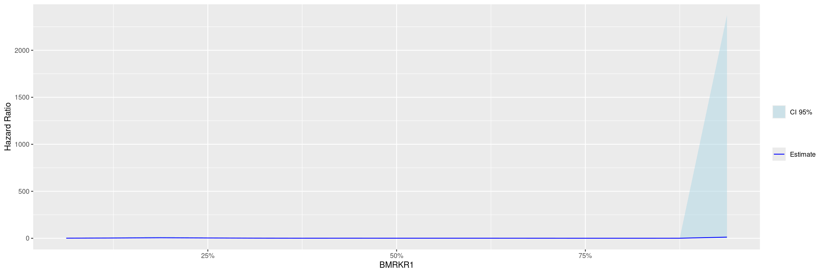
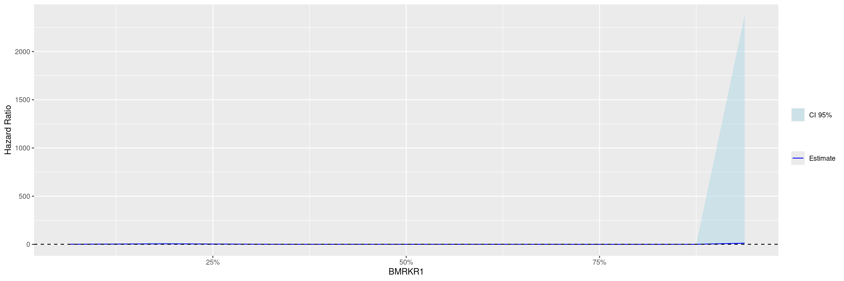
Before we can plot the data, the broom::tidy() method needs to be applied to the STEP result to obtain graph ready data. Thereafter with the g_step() function we can create a graph showing the estimated HR along the continuous biomarker subgroups.

Code

step_data <- broom::tidy(step_matrix)

graph <- g_step(step_data)

graph

We can also add a reference line.

Code

graph +
  geom_hline(aes(yintercept = 1), linetype = 2)

Code

sessionInfo()

R version 4.4.1 (2024-06-14)
Platform: x86_64-pc-linux-gnu
Running under: Ubuntu 22.04.4 LTS

Matrix products: default
BLAS:   /usr/lib/x86_64-linux-gnu/openblas-pthread/libblas.so.3 
LAPACK: /usr/lib/x86_64-linux-gnu/openblas-pthread/libopenblasp-r0.3.20.so;  LAPACK version 3.10.0

locale:
 [1] LC_CTYPE=en_US.UTF-8       LC_NUMERIC=C              
 [3] LC_TIME=en_US.UTF-8        LC_COLLATE=en_US.UTF-8    
 [5] LC_MONETARY=en_US.UTF-8    LC_MESSAGES=en_US.UTF-8   
 [7] LC_PAPER=en_US.UTF-8       LC_NAME=C                 
 [9] LC_ADDRESS=C               LC_TELEPHONE=C            
[11] LC_MEASUREMENT=en_US.UTF-8 LC_IDENTIFICATION=C       

time zone: Etc/UTC
tzcode source: system (glibc)

attached base packages:
[1] stats     graphics  grDevices utils     datasets  methods   base     

other attached packages:
[1] dplyr_1.1.4           ggplot2.utils_0.3.2   ggplot2_3.5.1        
[4] tern_0.9.5.9022       rtables_0.6.9.9014    magrittr_2.0.3       
[7] formatters_0.5.9.9001

loaded via a namespace (and not attached):
 [1] utf8_1.2.4                    generics_0.1.3               
 [3] tidyr_1.3.1                   EnvStats_3.0.0               
 [5] stringi_1.8.4                 lattice_0.22-6               
 [7] digest_0.6.37                 evaluate_0.24.0              
 [9] grid_4.4.1                    fastmap_1.2.0                
[11] jsonlite_1.8.8                Matrix_1.7-0                 
[13] backports_1.5.0               survival_3.7-0               
[15] purrr_1.0.2                   fansi_1.0.6                  
[17] scales_1.3.0                  codetools_0.2-20             
[19] Rdpack_2.6.1                  cli_3.6.3                    
[21] ggpp_0.5.8-1                  rlang_1.1.4                  
[23] rbibutils_2.2.16              munsell_0.5.1                
[25] splines_4.4.1                 withr_3.0.1                  
[27] yaml_2.3.10                   tools_4.4.1                  
[29] polynom_1.4-1                 checkmate_2.3.2              
[31] colorspace_2.1-1              forcats_1.0.0                
[33] ggstats_0.6.0                 broom_1.0.6                  
[35] vctrs_0.6.5                   R6_2.5.1                     
[37] lifecycle_1.0.4               stringr_1.5.1                
[39] htmlwidgets_1.6.4             MASS_7.3-61                  
[41] pkgconfig_2.0.3               pillar_1.9.0                 
[43] gtable_0.3.5                  glue_1.7.0                   
[45] xfun_0.47                     tibble_3.2.1                 
[47] tidyselect_1.2.1              knitr_1.48                   
[49] farver_2.1.2                  htmltools_0.5.8.1            
[51] labeling_0.4.3                rmarkdown_2.28               
[53] random.cdisc.data_0.3.15.9009 compiler_4.4.1

Reuse