RG2

Response Graphs by Treatment Arms

---

Setup

The same setup as in RG1 is used.

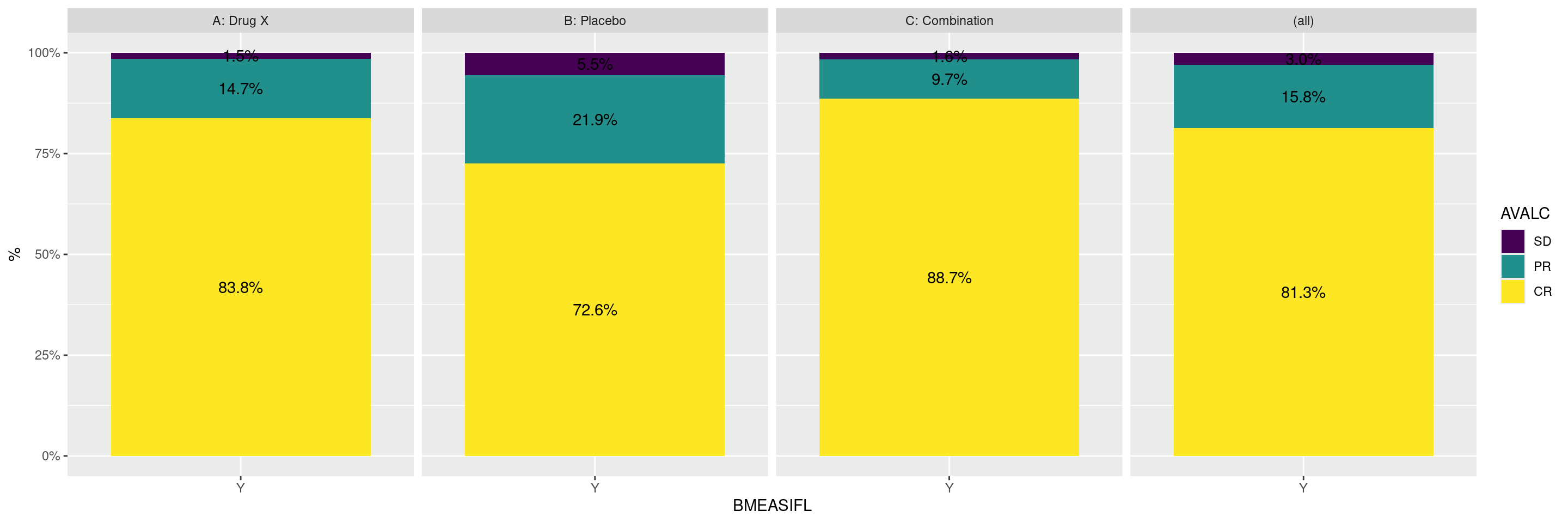
For ggplot() used in all analyses, we add by = BMEASIFL in the aesthetics to support the calculation of proportions using geom_text(stat = "prop").

library(tern)
library(ggplot2.utils)
library(dplyr)

adrs <- random.cdisc.data::cadrs %>%
  df_explicit_na() %>%
  mutate(AVALC = ordered(AVALC, levels = c("<Missing>", "NE", "PD", "SD", "PR", "CR"))) %>%
  filter(PARAMCD == "BESRSPI", BMEASIFL == "Y")

Plot

The facet_grid() layer from ggplot2 can be used to plot response by treatment arm and the margins argument can be used to produce the (all) column.

graph <- ggplot(adrs, aes(BMEASIFL, fill = AVALC, by = BMEASIFL)) +
  geom_bar(aes(BMEASIFL), position = "fill") +
  geom_text(stat = "prop", position = position_fill(.5)) +
  scale_y_continuous(labels = scales::percent) +
  ylab("%") +
  facet_grid(. ~ ARM, margins = TRUE)

graph

Session Info

sessionInfo()

R version 4.4.1 (2024-06-14)
Platform: x86_64-pc-linux-gnu
Running under: Ubuntu 22.04.4 LTS

Matrix products: default
BLAS:   /usr/lib/x86_64-linux-gnu/openblas-pthread/libblas.so.3 
LAPACK: /usr/lib/x86_64-linux-gnu/openblas-pthread/libopenblasp-r0.3.20.so;  LAPACK version 3.10.0

locale:
 [1] LC_CTYPE=en_US.UTF-8       LC_NUMERIC=C              
 [3] LC_TIME=en_US.UTF-8        LC_COLLATE=en_US.UTF-8    
 [5] LC_MONETARY=en_US.UTF-8    LC_MESSAGES=en_US.UTF-8   
 [7] LC_PAPER=en_US.UTF-8       LC_NAME=C                 
 [9] LC_ADDRESS=C               LC_TELEPHONE=C            
[11] LC_MEASUREMENT=en_US.UTF-8 LC_IDENTIFICATION=C       

time zone: Etc/UTC
tzcode source: system (glibc)

attached base packages:
[1] stats     graphics  grDevices utils     datasets  methods   base     

other attached packages:
[1] dplyr_1.1.4           ggplot2.utils_0.3.2   ggplot2_3.5.1        
[4] tern_0.9.5.9022       rtables_0.6.9.9014    magrittr_2.0.3       
[7] formatters_0.5.9.9001

loaded via a namespace (and not attached):
 [1] utf8_1.2.4                    generics_0.1.3               
 [3] tidyr_1.3.1                   EnvStats_3.0.0               
 [5] stringi_1.8.4                 lattice_0.22-6               
 [7] digest_0.6.37                 evaluate_0.24.0              
 [9] grid_4.4.1                    fastmap_1.2.0                
[11] jsonlite_1.8.8                Matrix_1.7-0                 
[13] backports_1.5.0               survival_3.7-0               
[15] purrr_1.0.2                   fansi_1.0.6                  
[17] viridisLite_0.4.2             scales_1.3.0                 
[19] codetools_0.2-20              Rdpack_2.6.1                 
[21] cli_3.6.3                     ggpp_0.5.8-1                 
[23] rlang_1.1.4                   rbibutils_2.2.16             
[25] munsell_0.5.1                 splines_4.4.1                
[27] withr_3.0.1                   yaml_2.3.10                  
[29] tools_4.4.1                   polynom_1.4-1                
[31] checkmate_2.3.2               colorspace_2.1-1             
[33] forcats_1.0.0                 ggstats_0.6.0                
[35] broom_1.0.6                   vctrs_0.6.5                  
[37] R6_2.5.1                      lifecycle_1.0.4              
[39] stringr_1.5.1                 htmlwidgets_1.6.4            
[41] MASS_7.3-61                   pkgconfig_2.0.3              
[43] pillar_1.9.0                  gtable_0.3.5                 
[45] glue_1.7.0                    xfun_0.47                    
[47] tibble_3.2.1                  tidyselect_1.2.1             
[49] knitr_1.48                    farver_2.1.2                 
[51] htmltools_0.5.8.1             labeling_0.4.3               
[53] rmarkdown_2.28                random.cdisc.data_0.3.15.9009
[55] compiler_4.4.1