DG1B

Histogram of One Numeric Variable by Treatment Arm

---

Setup

We will use the cadsl data set from the random.cdisc.data package and ggplot2 to create the plots. In this example, we will plot histograms of one or multiple numeric variables. We start by selecting the biomarker evaluable population with the flag variable BEP01FL and then populating a new continuous biomarker variable, BMRKR3.

library(tern)
library(ggplot2.utils)
library(dplyr)
library(tibble)
library(tidyr)

adsl <- random.cdisc.data::cadsl %>%
  df_explicit_na() %>%
  filter(BEP01FL == "Y") %>%
  mutate(BMRKR3 = rnorm(n(), mean = 7, sd = 2))

Plot

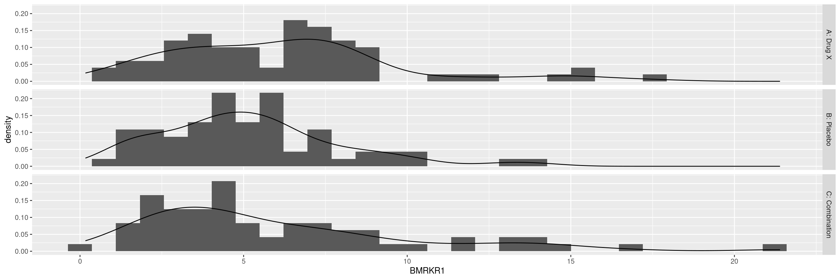
Below example shows histograms for the BMRKR1 variable by treatment ARM. Including a statistics table in this graph works in the same way as we did above for DG1A.

graph <- ggplot(adsl, aes(BMRKR1)) +
  geom_histogram(aes(y = after_stat(density)), bins = 30) +
  geom_density(aes(y = after_stat(density))) +
  facet_grid(ARM ~ .)

graph

Session Info

sessionInfo()

R version 4.4.1 (2024-06-14)
Platform: x86_64-pc-linux-gnu
Running under: Ubuntu 22.04.4 LTS

Matrix products: default
BLAS:   /usr/lib/x86_64-linux-gnu/openblas-pthread/libblas.so.3 
LAPACK: /usr/lib/x86_64-linux-gnu/openblas-pthread/libopenblasp-r0.3.20.so;  LAPACK version 3.10.0

locale:
 [1] LC_CTYPE=en_US.UTF-8       LC_NUMERIC=C              
 [3] LC_TIME=en_US.UTF-8        LC_COLLATE=en_US.UTF-8    
 [5] LC_MONETARY=en_US.UTF-8    LC_MESSAGES=en_US.UTF-8   
 [7] LC_PAPER=en_US.UTF-8       LC_NAME=C                 
 [9] LC_ADDRESS=C               LC_TELEPHONE=C            
[11] LC_MEASUREMENT=en_US.UTF-8 LC_IDENTIFICATION=C       

time zone: Etc/UTC
tzcode source: system (glibc)

attached base packages:
[1] stats     graphics  grDevices utils     datasets  methods   base     

other attached packages:
[1] tidyr_1.3.1           tibble_3.2.1          dplyr_1.1.4          
[4] ggplot2.utils_0.3.2   ggplot2_3.5.1         tern_0.9.5.9022      
[7] rtables_0.6.9.9014    magrittr_2.0.3        formatters_0.5.9.9001

loaded via a namespace (and not attached):
 [1] utf8_1.2.4                    generics_0.1.3               
 [3] EnvStats_3.0.0                stringi_1.8.4                
 [5] lattice_0.22-6                digest_0.6.37                
 [7] evaluate_0.24.0               grid_4.4.1                   
 [9] fastmap_1.2.0                 jsonlite_1.8.8               
[11] Matrix_1.7-0                  backports_1.5.0              
[13] survival_3.7-0                purrr_1.0.2                  
[15] fansi_1.0.6                   scales_1.3.0                 
[17] codetools_0.2-20              Rdpack_2.6.1                 
[19] cli_3.6.3                     ggpp_0.5.8-1                 
[21] rlang_1.1.4                   rbibutils_2.2.16             
[23] munsell_0.5.1                 splines_4.4.1                
[25] withr_3.0.1                   yaml_2.3.10                  
[27] tools_4.4.1                   polynom_1.4-1                
[29] checkmate_2.3.2               colorspace_2.1-1             
[31] forcats_1.0.0                 ggstats_0.6.0                
[33] broom_1.0.6                   vctrs_0.6.5                  
[35] R6_2.5.1                      lifecycle_1.0.4              
[37] stringr_1.5.1                 htmlwidgets_1.6.4            
[39] MASS_7.3-61                   pkgconfig_2.0.3              
[41] pillar_1.9.0                  gtable_0.3.5                 
[43] glue_1.7.0                    xfun_0.47                    
[45] tidyselect_1.2.1              knitr_1.48                   
[47] farver_2.1.2                  htmltools_0.5.8.1            
[49] labeling_0.4.3                rmarkdown_2.28               
[51] random.cdisc.data_0.3.15.9009 compiler_4.4.1