KG1B

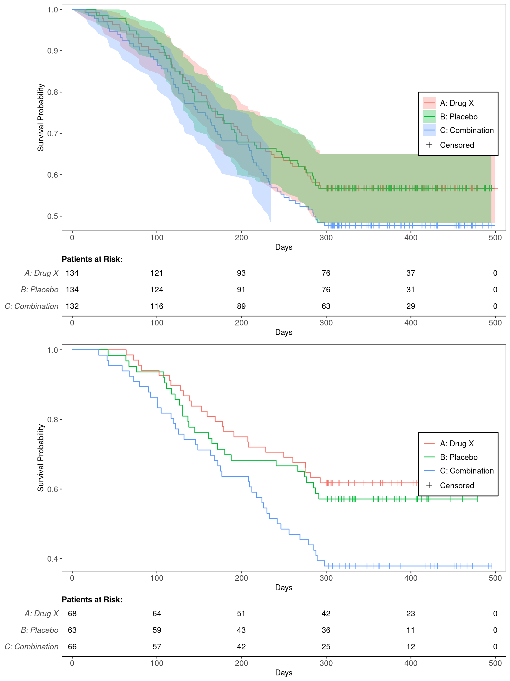
Kaplan-Meier Graph for Comparing ITT and BEP Populations

We will use the cadtte data set from the random.cdisc.data package to create the Kaplan-Meier (KM) plots. We start by filtering the time-to-event dataset for the overall survival observations and by one treatment arm (A), creating a new variable for event information, and curating a list of variables required to produce the plot.

Code

library(tern)
library(dplyr)
library(ggplot2)
library(grid)

adtte_arm <- random.cdisc.data::cadtte %>%
  df_explicit_na() %>%
  filter(PARAMCD == "OS", ARM == "A: Drug X") %>%
  mutate(is_event = CNSR == 0)

variables <- list(tte = "AVAL", is_event = "is_event", arm = "ARM")

Here we only filter the time-to-event dataset for the overall survival observations, but keep all treatment arms and the overall population.

Code

adtte <- random.cdisc.data::cadtte %>%
  df_explicit_na() %>%
  filter(PARAMCD == "OS") %>%
  mutate(is_event = CNSR == 0)

variables <- list(tte = "AVAL", is_event = "is_event", arm = "ARM")

Plot the ITT (top, with CIs) and BEP (bottom, without CIs) KM graphs, convert them to ggplotGrob objects, and combine the plots via rbind. Then, use the grid package to create an empty plot area, and draw the KM curves on the graph device.

Code

res1 <- g_km(
  df = adtte, variables = variables, annot_surv_med = FALSE, ci_ribbon = TRUE
)

res2 <- g_km(
  df = filter(adtte, BEP01FL == "Y"), variables = variables, annot_surv_med = FALSE
)

g <- rbind(ggplot2::ggplotGrob(res1), ggplot2::ggplotGrob(res2), size = "first")

grid.newpage()
grid.draw(g)

Code

sessionInfo()

R version 4.4.1 (2024-06-14)
Platform: x86_64-pc-linux-gnu
Running under: Ubuntu 22.04.4 LTS

Matrix products: default
BLAS:   /usr/lib/x86_64-linux-gnu/openblas-pthread/libblas.so.3 
LAPACK: /usr/lib/x86_64-linux-gnu/openblas-pthread/libopenblasp-r0.3.20.so;  LAPACK version 3.10.0

locale:
 [1] LC_CTYPE=en_US.UTF-8       LC_NUMERIC=C              
 [3] LC_TIME=en_US.UTF-8        LC_COLLATE=en_US.UTF-8    
 [5] LC_MONETARY=en_US.UTF-8    LC_MESSAGES=en_US.UTF-8   
 [7] LC_PAPER=en_US.UTF-8       LC_NAME=C                 
 [9] LC_ADDRESS=C               LC_TELEPHONE=C            
[11] LC_MEASUREMENT=en_US.UTF-8 LC_IDENTIFICATION=C       

time zone: Etc/UTC
tzcode source: system (glibc)

attached base packages:
[1] grid      stats     graphics  grDevices utils     datasets  methods  
[8] base     

other attached packages:
[1] ggplot2_3.5.1         dplyr_1.1.4           tern_0.9.5.9022      
[4] rtables_0.6.9.9014    magrittr_2.0.3        formatters_0.5.9.9001

loaded via a namespace (and not attached):
 [1] Matrix_1.7-0                  gtable_0.3.5                 
 [3] jsonlite_1.8.8                compiler_4.4.1               
 [5] tidyselect_1.2.1              stringr_1.5.1                
 [7] tidyr_1.3.1                   splines_4.4.1                
 [9] scales_1.3.0                  yaml_2.3.10                  
[11] fastmap_1.2.0                 lattice_0.22-6               
[13] R6_2.5.1                      labeling_0.4.3               
[15] generics_0.1.3                knitr_1.48                   
[17] forcats_1.0.0                 rbibutils_2.2.16             
[19] htmlwidgets_1.6.4             backports_1.5.0              
[21] checkmate_2.3.2               tibble_3.2.1                 
[23] munsell_0.5.1                 pillar_1.9.0                 
[25] rlang_1.1.4                   utf8_1.2.4                   
[27] broom_1.0.6                   stringi_1.8.4                
[29] xfun_0.47                     cli_3.6.3                    
[31] withr_3.0.1                   Rdpack_2.6.1                 
[33] digest_0.6.37                 cowplot_1.1.3                
[35] lifecycle_1.0.4               vctrs_0.6.5                  
[37] evaluate_0.24.0               glue_1.7.0                   
[39] farver_2.1.2                  codetools_0.2-20             
[41] survival_3.7-0                random.cdisc.data_0.3.15.9009
[43] fansi_1.0.6                   colorspace_2.1-1             
[45] purrr_1.0.2                   rmarkdown_2.28               
[47] tools_4.4.1                   pkgconfig_2.0.3              
[49] htmltools_0.5.8.1

Reuse