AG1
AG
In this page we collect standard utilities for plotting which can be applied in principle to all graphs. Then we don’t need to repeat explaining these in each of the other…
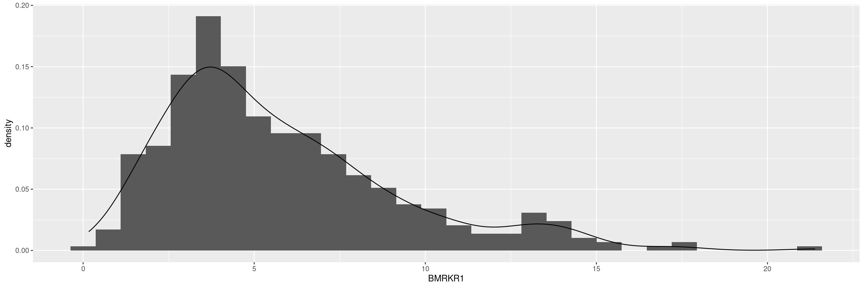
This is a collection of Biomarker Analysis graph templates.