RFG2B
Response Forest Graphs for Comparing Continuous Biomarker Effects Across Subgroups (Multiple Continuous Biomarkers by Manual Subgroup Categories)
These templates are helpful when we are interested in modelling the effects of continuous biomarker variables on the binary response outcome, conditional on covariates and/or stratification variables included in (conditional) logistic regression models. We would like to assess how the estimates effects change when we look at different subgroups.
In detail the differences to RFG1 are the following:
- The
extract_rsp_subgroups()andtabulate_rsp_subgroups()functions used in RFG1 evaluate the treatment effects from two arms, across subgroups. On the other hand, theextract_rsp_biomarkers()andtabulate_rsp_biomarkers()functions used here in RFG2 evaluate the effects from continuous biomarkers on the probability for response. - The
extract_rsp_subgroups()andtabulate_rsp_subgroups()functions only allow specification of a single treatment arm variable, while theextract_rsp_biomarkers()andtabulate_rsp_biomarkers()allow to look at multiple continuous biomarker variables at once. - In addition to the treatment arms, the use of
extract_rsp_subgroups()andtabulate_rsp_subgroups()functions can be extended to other binary variables. For example, we could define the binarizedARMvariable asAGE>=65vs.AGE<65and then look at the odds ratios across subgroups. For theextract_rsp_biomarkers()andtabulate_rsp_biomarkers()functions, we could use the original continuous biomarker variableAGE, and then look at the estimated effect across subgroups.
Similarly like in RFG1, we will use the cadrs data set from the random.cdisc.data package. Here we just filter for the Best Confirmed Overall Response by Investigator and patients with measurable disease at baseline, and define a new variable COMPRESP to include complete responses only.
It is also possible to join and select subgroup categories manually using the groups_lists argument, as follows.
Code
df <- extract_rsp_biomarkers(
  variables = list(
    rsp = "COMPRESP",
    biomarkers = c("BMRKR1", "AGE"),
    covariates = "SEX",
    subgroups = "BMRKR2"
  ),
  data = adrs_f,
  groups_list = list(
    BMRKR2 = list(
      one = c("LOW", "MEDIUM"),
      two = "HIGH"
    )
  )
)

result <- tabulate_rsp_biomarkers(df, vars = c("n_tot", "n_rsp", "prop", "or", "ci"))
g_forest(result, xlim = c(0.7, 1.4))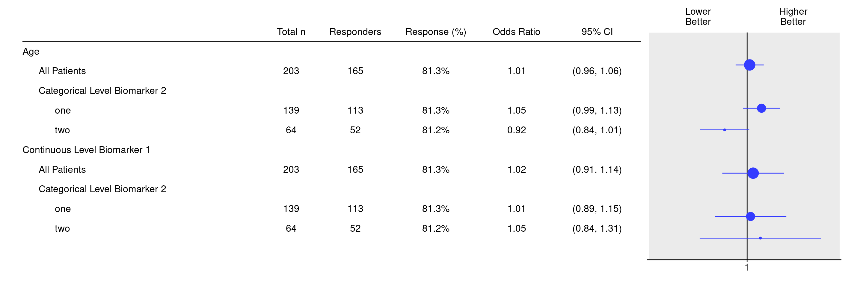
R version 4.4.1 (2024-06-14)
Platform: x86_64-pc-linux-gnu
Running under: Ubuntu 22.04.4 LTS

Matrix products: default
BLAS:   /usr/lib/x86_64-linux-gnu/openblas-pthread/libblas.so.3
LAPACK: /usr/lib/x86_64-linux-gnu/openblas-pthread/libopenblasp-r0.3.20.so;  LAPACK version 3.10.0

locale:
 [1] LC_CTYPE=en_US.UTF-8       LC_NUMERIC=C
 [3] LC_TIME=en_US.UTF-8        LC_COLLATE=en_US.UTF-8
 [5] LC_MONETARY=en_US.UTF-8    LC_MESSAGES=en_US.UTF-8
 [7] LC_PAPER=en_US.UTF-8       LC_NAME=C
 [9] LC_ADDRESS=C               LC_TELEPHONE=C
[11] LC_MEASUREMENT=en_US.UTF-8 LC_IDENTIFICATION=C

time zone: Etc/UTC
tzcode source: system (glibc)

attached base packages:
[1] stats4    stats     graphics  grDevices utils     datasets  methods
[8] base

other attached packages:
 [1] hermes_1.7.2.9002           SummarizedExperiment_1.34.0
 [3] Biobase_2.64.0              GenomicRanges_1.56.1
 [5] GenomeInfoDb_1.40.1         IRanges_2.38.1
 [7] S4Vectors_0.42.1            BiocGenerics_0.50.0
 [9] MatrixGenerics_1.16.0       matrixStats_1.4.1
[11] ggfortify_0.4.17            ggplot2_3.5.1
[13] dplyr_1.1.4                 tern_0.9.5.9022
[15] rtables_0.6.9.9014          magrittr_2.0.3
[17] formatters_0.5.9.9001

loaded via a namespace (and not attached):
  [1] Rdpack_2.6.1                  DBI_1.2.3
  [3] httr2_1.0.3                   gridExtra_2.3
  [5] biomaRt_2.60.1                rlang_1.1.4
  [7] clue_0.3-65                   GetoptLong_1.0.5
  [9] compiler_4.4.1                RSQLite_2.3.7
 [11] png_0.1-8                     vctrs_0.6.5
 [13] stringr_1.5.1                 pkgconfig_2.0.3
 [15] shape_1.4.6.1                 crayon_1.5.3
 [17] fastmap_1.2.0                 dbplyr_2.5.0
 [19] backports_1.5.0               XVector_0.44.0
 [21] labeling_0.4.3                utf8_1.2.4
 [23] rmarkdown_2.28                UCSC.utils_1.0.0
 [25] purrr_1.0.2                   bit_4.0.5
 [27] xfun_0.47                     MultiAssayExperiment_1.30.3
 [29] zlibbioc_1.50.0               cachem_1.1.0
 [31] jsonlite_1.8.8                progress_1.2.3
 [33] blob_1.2.4                    DelayedArray_0.30.1
 [35] prettyunits_1.2.0             broom_1.0.6
 [37] parallel_4.4.1                cluster_2.1.6
 [39] R6_2.5.1                      stringi_1.8.4
 [41] RColorBrewer_1.1-3            Rcpp_1.0.13
 [43] assertthat_0.2.1              iterators_1.0.14
 [45] knitr_1.48                    Matrix_1.7-0
 [47] splines_4.4.1                 tidyselect_1.2.1
 [49] abind_1.4-8                   yaml_2.3.10
 [51] doParallel_1.0.17             codetools_0.2-20
 [53] curl_5.2.2                    lattice_0.22-6
 [55] tibble_3.2.1                  withr_3.0.1
 [57] KEGGREST_1.44.1               evaluate_0.24.0
 [59] survival_3.7-0                BiocFileCache_2.12.0
 [61] xml2_1.3.6                    circlize_0.4.16
 [63] Biostrings_2.72.1             filelock_1.0.3
 [65] pillar_1.9.0                  checkmate_2.3.2
 [67] foreach_1.5.2                 generics_0.1.3
 [69] hms_1.1.3                     munsell_0.5.1
 [71] scales_1.3.0                  glue_1.7.0
 [73] tools_4.4.1                   forcats_1.0.0
 [75] cowplot_1.1.3                 grid_4.4.1
 [77] tidyr_1.3.1                   rbibutils_2.2.16
 [79] AnnotationDbi_1.66.0          colorspace_2.1-1
 [81] random.cdisc.data_0.3.15.9009 GenomeInfoDbData_1.2.12
 [83] cli_3.6.3                     rappdirs_0.3.3
 [85] fansi_1.0.6                   S4Arrays_1.4.1
 [87] ComplexHeatmap_2.20.0         gtable_0.3.5
 [89] digest_0.6.37                 SparseArray_1.4.8
 [91] ggrepel_0.9.6                 farver_2.1.2
 [93] rjson_0.2.22                  htmlwidgets_1.6.4
 [95] memoise_2.0.1                 htmltools_0.5.8.1
 [97] lifecycle_1.0.4               httr_1.4.7
 [99] GlobalOptions_0.1.2           bit64_4.0.5