DG1A

Histograms of Two Numeric Variables

We will use the cadsl data set from the random.cdisc.data package and ggplot2 to create the plots. In this example, we will plot histograms of one or multiple numeric variables. We start by selecting the biomarker evaluable population with the flag variable BEP01FL and then populating a new continuous biomarker variable, BMRKR3.

Code

library(tern)
library(ggplot2.utils)
library(dplyr)
library(tibble)
library(tidyr)

adsl <- random.cdisc.data::cadsl %>%
  df_explicit_na() %>%
  filter(BEP01FL == "Y") %>%
  mutate(BMRKR3 = rnorm(n(), mean = 7, sd = 2))

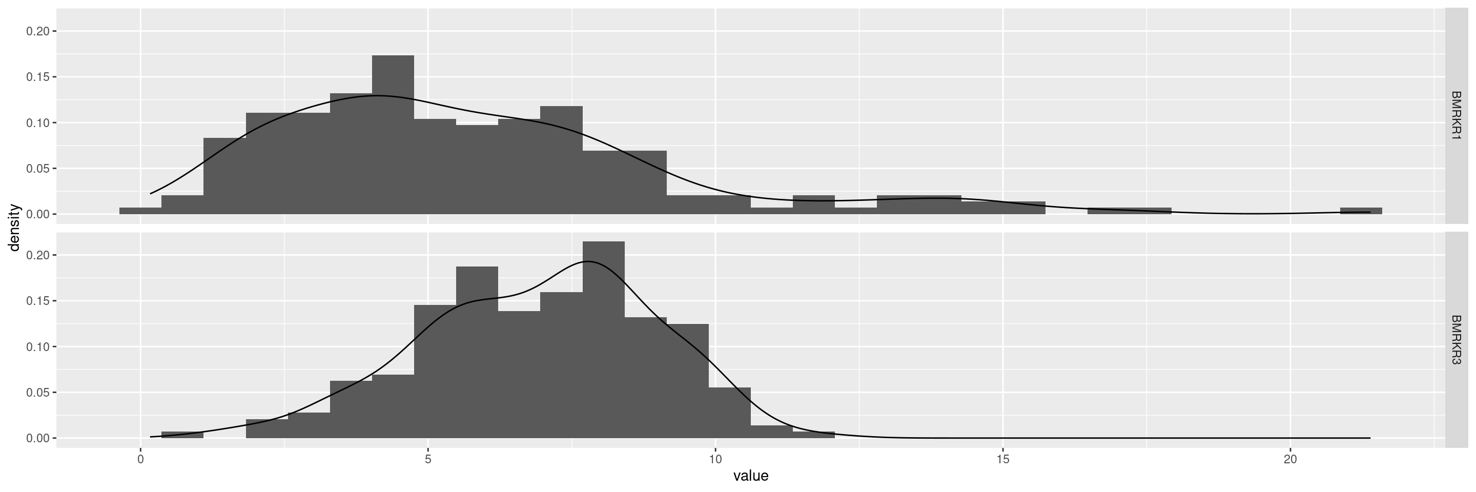
In this example, we will manipulate the variables that we want to show in the graph into a long data format using the pivot_longer() function from tidyr. This is necessary such that below we can use the faceting layer facet_grid() to plot each variable in its own facet.

Code

num_var_long <- adsl %>%
  pivot_longer(
    c(BMRKR1, BMRKR3),
    names_to = "var",
    values_to = "value"
  ) %>%
  select(var, value)

Producing the base plot is then simple: We use the same code as above but just add the faceting layer.

Code

graph <- ggplot(num_var_long, aes(value)) +
  geom_histogram(aes(y = after_stat(density)), bins = 30) +
  geom_density(aes(y = after_stat(density))) +
  facet_grid(var ~ .)

graph

Similar to the DG1 example, we will calculate and populate the statistics table to accompany the plot. Note that also here we can use the pivot_longer() function to also obtain the statistics table input orig_tb and then data_tb in long format, and thus parallel to the biomarker variable format in num_var_long.

Code

orig_tb <- num_var_long %>%
  group_by(var) %>%
  summarize_at("value", list(mean = mean, median = median)) %>%
  pivot_longer(
    c(mean, median),
    names_to = "Statistic",
    values_to = "Value"
  )

data_tb <- orig_tb %>%
  group_by(var) %>%
  summarize(x = 1, y = 1, tb = list(tibble(Statistic, Value)))

graph <- graph +
  geom_table_npc(data = data_tb, aes(npcx = x, npcy = y, label = tb))

graph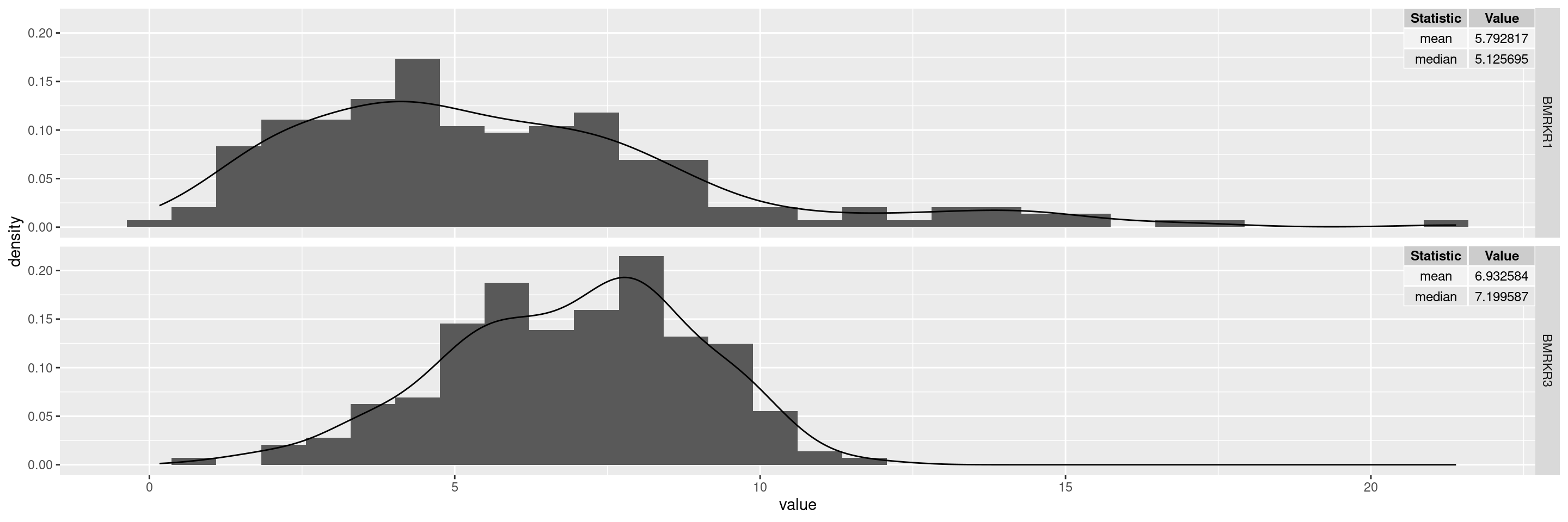

Code

sessionInfo()

R version 4.4.1 (2024-06-14)
Platform: x86_64-pc-linux-gnu
Running under: Ubuntu 22.04.4 LTS

Matrix products: default
BLAS:   /usr/lib/x86_64-linux-gnu/openblas-pthread/libblas.so.3 
LAPACK: /usr/lib/x86_64-linux-gnu/openblas-pthread/libopenblasp-r0.3.20.so;  LAPACK version 3.10.0

locale:
 [1] LC_CTYPE=en_US.UTF-8       LC_NUMERIC=C              
 [3] LC_TIME=en_US.UTF-8        LC_COLLATE=en_US.UTF-8    
 [5] LC_MONETARY=en_US.UTF-8    LC_MESSAGES=en_US.UTF-8   
 [7] LC_PAPER=en_US.UTF-8       LC_NAME=C                 
 [9] LC_ADDRESS=C               LC_TELEPHONE=C            
[11] LC_MEASUREMENT=en_US.UTF-8 LC_IDENTIFICATION=C       

time zone: Etc/UTC
tzcode source: system (glibc)

attached base packages:
[1] stats     graphics  grDevices utils     datasets  methods   base     

other attached packages:
[1] tidyr_1.3.1           tibble_3.2.1          dplyr_1.1.4          
[4] ggplot2.utils_0.3.2   ggplot2_3.5.1         tern_0.9.5.9022      
[7] rtables_0.6.9.9014    magrittr_2.0.3        formatters_0.5.9.9001

loaded via a namespace (and not attached):
 [1] utf8_1.2.4                    generics_0.1.3               
 [3] EnvStats_3.0.0                stringi_1.8.4                
 [5] lattice_0.22-6                digest_0.6.37                
 [7] evaluate_0.24.0               grid_4.4.1                   
 [9] fastmap_1.2.0                 jsonlite_1.8.8               
[11] Matrix_1.7-0                  backports_1.5.0              
[13] survival_3.7-0                gridExtra_2.3                
[15] purrr_1.0.2                   fansi_1.0.6                  
[17] scales_1.3.0                  codetools_0.2-20             
[19] Rdpack_2.6.1                  cli_3.6.3                    
[21] ggpp_0.5.8-1                  rlang_1.1.4                  
[23] rbibutils_2.2.16              munsell_0.5.1                
[25] splines_4.4.1                 withr_3.0.1                  
[27] yaml_2.3.10                   tools_4.4.1                  
[29] polynom_1.4-1                 checkmate_2.3.2              
[31] colorspace_2.1-1              forcats_1.0.0                
[33] ggstats_0.6.0                 broom_1.0.6                  
[35] vctrs_0.6.5                   R6_2.5.1                     
[37] lifecycle_1.0.4               stringr_1.5.1                
[39] htmlwidgets_1.6.4             MASS_7.3-61                  
[41] pkgconfig_2.0.3               pillar_1.9.0                 
[43] gtable_0.3.5                  glue_1.7.0                   
[45] xfun_0.47                     tidyselect_1.2.1             
[47] knitr_1.48                    farver_2.1.2                 
[49] htmltools_0.5.8.1             labeling_0.4.3               
[51] rmarkdown_2.28                random.cdisc.data_0.3.15.9009
[53] compiler_4.4.1

Reuse