Biomarker Analysis Catalog - Dev
  • Dev
    • Stable
  1. Graphs
  2. SFG
  3. SFG5
  4. SFG5A
  • Index

  • Tables
    • CPMT
      • CPMT1
      • CPMT2
        • CPMT2A
      • CPMT3
    • DT
      • DT1
        • DT1A
        • DT1B
        • DT1C
      • DT2
        • DT2A
    • TET
      • TET1
        • TET1A

  • Graphs
    • AG
      • AG1
    • DG
      • DG1
        • DG1A
        • DG1B
      • DG2
      • DG3
        • DG3A
      • DG4
    • KG
      • KG1
        • KG1A
        • KG1B
      • KG2
        • KG2A
      • KG3
      • KG4
        • KG4A
        • KG4B
      • KG5
        • KG5A
        • KG5B
    • RFG
      • RFG1
        • RFG1A
      • RFG2
        • RFG2A
        • RFG2B
        • RFG2C
      • RFG3
    • RG
      • RG1
        • RG1A
        • RG1B
        • RG1C
      • RG2
        • RG2A
      • RG3
        • RG3A
        • RG3B
    • SPG
      • SPG1
      • SPG2
    • RNAG
      • RNAG1
      • RNAG2
      • RNAG3
      • RNAG4
      • RNAG5
      • RNAG6
      • RNAG7
      • RNAG8
      • RNAG9
      • RNAG10
    • SFG
      • SFG1
        • SFG1A
        • SFG1B
      • SFG2
        • SFG2A
        • SFG2B
        • SFG2C
        • SFG2D
      • SFG3
        • SFG3A
      • SFG4
      • SFG5
        • SFG5A
        • SFG5B
        • SFG5C
      • SFG6
        • SFG6A
        • SFG6B
        • SFG6C
  1. Graphs
  2. SFG
  3. SFG5
  4. SFG5A

SFG5A

Survival Forest Graph Comparing Categorical Biomarker Groups on Subgroups

SFG

  • Setup
  • Plot
  • Session Info

We prepare the data similarly as in SFG1.

Code
library(tern)
library(dplyr)

AGE_probs <- 0.5

adtte <- random.cdisc.data::cadtte %>%
  df_explicit_na() %>%
  filter(
    PARAMCD == "OS"
  ) %>%
  mutate(
    AVAL = day2month(AVAL),
    AVALU = "Months",
    is_event = CNSR == 0,
    ARM_BIN = fct_collapse_only(
      ARM,
      CTRL = "B: Placebo",
      TRT = c("A: Drug X", "C: Combination")
    ),
    AGE_BIN = cut_quantile_bins(AGE, probs = AGE_probs),
    BMRKR2 = fct_explicit_na_if(BMRKR2, BEP01FL == "N"),
    BMRKR2_BIN = fct_collapse_only(
      BMRKR2,
      High = "HIGH",
      Low = c("MEDIUM", "LOW")
    )
  ) %>%
  var_relabel(
    BEP01FL = "BEP",
    BMRKR2_BIN = "Biomarker (Binary)"
  )

The main difference here is that we ensure that col_info is aligned across all subtables before using rbind() to combine subtables. (Generally this is worth trying out if the rbind() does not work out of the box to combine subtables.)

Code
tables_all <- function(filter_var, filter_condition, sub_var) {
  dataset <- adtte %>%
    filter(!!as.name(filter_var) == filter_condition)
  if (nrow(dataset) == 0) {
    stop(paste("Subset", filter_var, "==", filter_condition, "is empty"))
  }
  tbl <- extract_survival_subgroups(
    variables = list(
      tte = "AVAL",
      is_event = "is_event",
      arm = "ARM_BIN",
      subgroups = sub_var
    ),
    label_all = "ITT",
    data = dataset
  )
  basic_table() %>%
    tabulate_survival_subgroups(
      df = tbl,
      vars = c("n_tot_events", "n", "n_events", "median", "hr", "ci"),
      time_unit = dataset$AVALU[1]
    )
}

add_subtitle <- function(sub_tab, sub_title) {
  label_at_path(sub_tab, path = row_paths(sub_tab)[[1]][1]) <- sub_title
  sub_tab
}

tables_list <- list(
  tables_all(filter_var = "BMRKR2_BIN", filter_condition = "High", sub_var = "SEX"),
  tables_all(filter_var = "BMRKR2_BIN", filter_condition = "Low", sub_var = "SEX"),
  tables_all(filter_var = "BMRKR2_BIN", filter_condition = "High", sub_var = "AGE_BIN"),
  tables_all(filter_var = "BMRKR2_BIN", filter_condition = "Low", sub_var = "AGE_BIN")
)
col_info(tables_list[[2]]) <- col_info(tables_list[[1]])
result <- rbind(
  add_subtitle(tables_list[[1]], "BMRKR2_BIN = High"),
  add_subtitle(tables_list[[2]], "BMRKR2_BIN = Low"),
  add_subtitle(tables_list[[3]], "BMRKR2_BIN = High"),
  add_subtitle(tables_list[[4]], "BMRKR2_BIN = Low")
)

We can now produce the forest plot using the g_forest() function.

Code
one_table <- tables_list[[1]]
g_forest(
  result,
  col_x = attr(one_table, "col_x"),
  col_ci = attr(one_table, "col_ci"),
  forest_header = attr(one_table, "forest_header"),
  col_symbol_size = attr(one_table, "col_symbol_size")
)

Code
sessionInfo()
R version 4.4.1 (2024-06-14)
Platform: x86_64-pc-linux-gnu
Running under: Ubuntu 22.04.4 LTS

Matrix products: default
BLAS:   /usr/lib/x86_64-linux-gnu/openblas-pthread/libblas.so.3 
LAPACK: /usr/lib/x86_64-linux-gnu/openblas-pthread/libopenblasp-r0.3.20.so;  LAPACK version 3.10.0

locale:
 [1] LC_CTYPE=en_US.UTF-8       LC_NUMERIC=C              
 [3] LC_TIME=en_US.UTF-8        LC_COLLATE=en_US.UTF-8    
 [5] LC_MONETARY=en_US.UTF-8    LC_MESSAGES=en_US.UTF-8   
 [7] LC_PAPER=en_US.UTF-8       LC_NAME=C                 
 [9] LC_ADDRESS=C               LC_TELEPHONE=C            
[11] LC_MEASUREMENT=en_US.UTF-8 LC_IDENTIFICATION=C       

time zone: Etc/UTC
tzcode source: system (glibc)

attached base packages:
[1] stats     graphics  grDevices utils     datasets  methods   base     

other attached packages:
[1] dplyr_1.1.4           tern_0.9.5.9022       rtables_0.6.9.9014   
[4] magrittr_2.0.3        formatters_0.5.9.9001

loaded via a namespace (and not attached):
 [1] Matrix_1.7-0                  gtable_0.3.5                 
 [3] jsonlite_1.8.8                compiler_4.4.1               
 [5] tidyselect_1.2.1              stringr_1.5.1                
 [7] tidyr_1.3.1                   splines_4.4.1                
 [9] scales_1.3.0                  yaml_2.3.10                  
[11] fastmap_1.2.0                 lattice_0.22-6               
[13] ggplot2_3.5.1                 R6_2.5.1                     
[15] labeling_0.4.3                generics_0.1.3               
[17] knitr_1.48                    forcats_1.0.0                
[19] rbibutils_2.2.16              htmlwidgets_1.6.4            
[21] backports_1.5.0               checkmate_2.3.2              
[23] tibble_3.2.1                  munsell_0.5.1                
[25] pillar_1.9.0                  rlang_1.1.4                  
[27] utf8_1.2.4                    broom_1.0.6                  
[29] stringi_1.8.4                 xfun_0.47                    
[31] cli_3.6.3                     withr_3.0.1                  
[33] Rdpack_2.6.1                  digest_0.6.37                
[35] grid_4.4.1                    cowplot_1.1.3                
[37] lifecycle_1.0.4               vctrs_0.6.5                  
[39] evaluate_0.24.0               glue_1.7.0                   
[41] farver_2.1.2                  codetools_0.2-20             
[43] survival_3.7-0                random.cdisc.data_0.3.15.9009
[45] fansi_1.0.6                   colorspace_2.1-1             
[47] purrr_1.0.2                   rmarkdown_2.28               
[49] tools_4.4.1                   pkgconfig_2.0.3              
[51] htmltools_0.5.8.1            

Reuse

Copyright 2023, Hoffmann-La Roche Ltd.
SFG5
SFG5B
Source Code
---
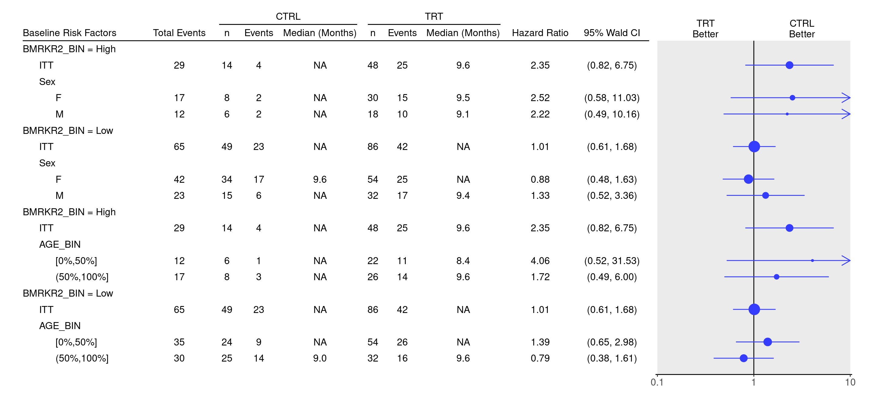
title: SFG5A
subtitle: Survival Forest Graph Comparing Categorical Biomarker Groups on Subgroups
categories: [SFG]
---

------------------------------------------------------------------------

::: panel-tabset
{{< include setup.qmd >}}

## Plot

The main difference here is that we ensure that `col_info` is aligned across all subtables before using `rbind()` to combine subtables.
(Generally this is worth trying out if the `rbind()` does not work out of the box to combine subtables.)

```{r}
tables_all <- function(filter_var, filter_condition, sub_var) {
  dataset <- adtte %>%
    filter(!!as.name(filter_var) == filter_condition)
  if (nrow(dataset) == 0) {
    stop(paste("Subset", filter_var, "==", filter_condition, "is empty"))
  }
  tbl <- extract_survival_subgroups(
    variables = list(
      tte = "AVAL",
      is_event = "is_event",
      arm = "ARM_BIN",
      subgroups = sub_var
    ),
    label_all = "ITT",
    data = dataset
  )
  basic_table() %>%
    tabulate_survival_subgroups(
      df = tbl,
      vars = c("n_tot_events", "n", "n_events", "median", "hr", "ci"),
      time_unit = dataset$AVALU[1]
    )
}

add_subtitle <- function(sub_tab, sub_title) {
  label_at_path(sub_tab, path = row_paths(sub_tab)[[1]][1]) <- sub_title
  sub_tab
}

tables_list <- list(
  tables_all(filter_var = "BMRKR2_BIN", filter_condition = "High", sub_var = "SEX"),
  tables_all(filter_var = "BMRKR2_BIN", filter_condition = "Low", sub_var = "SEX"),
  tables_all(filter_var = "BMRKR2_BIN", filter_condition = "High", sub_var = "AGE_BIN"),
  tables_all(filter_var = "BMRKR2_BIN", filter_condition = "Low", sub_var = "AGE_BIN")
)
col_info(tables_list[[2]]) <- col_info(tables_list[[1]])
result <- rbind(
  add_subtitle(tables_list[[1]], "BMRKR2_BIN = High"),
  add_subtitle(tables_list[[2]], "BMRKR2_BIN = Low"),
  add_subtitle(tables_list[[3]], "BMRKR2_BIN = High"),
  add_subtitle(tables_list[[4]], "BMRKR2_BIN = Low")
)
```

We can now produce the forest plot using the `g_forest()` function.

```{r, fig.width = 15, fig.height = 7}
one_table <- tables_list[[1]]
g_forest(
  result,
  col_x = attr(one_table, "col_x"),
  col_ci = attr(one_table, "col_ci"),
  forest_header = attr(one_table, "forest_header"),
  col_symbol_size = attr(one_table, "col_symbol_size")
)
```

{{< include ../../misc/session_info.qmd >}}
:::

Made with ❤️ by the Statistical Engineering Team StatisticalEngineering

  • License

  • Edit this page
  • Report an issue
Cookie Preferences