KG1

Kaplan-Meier Graphs for One Treatment Arm

---

Setup

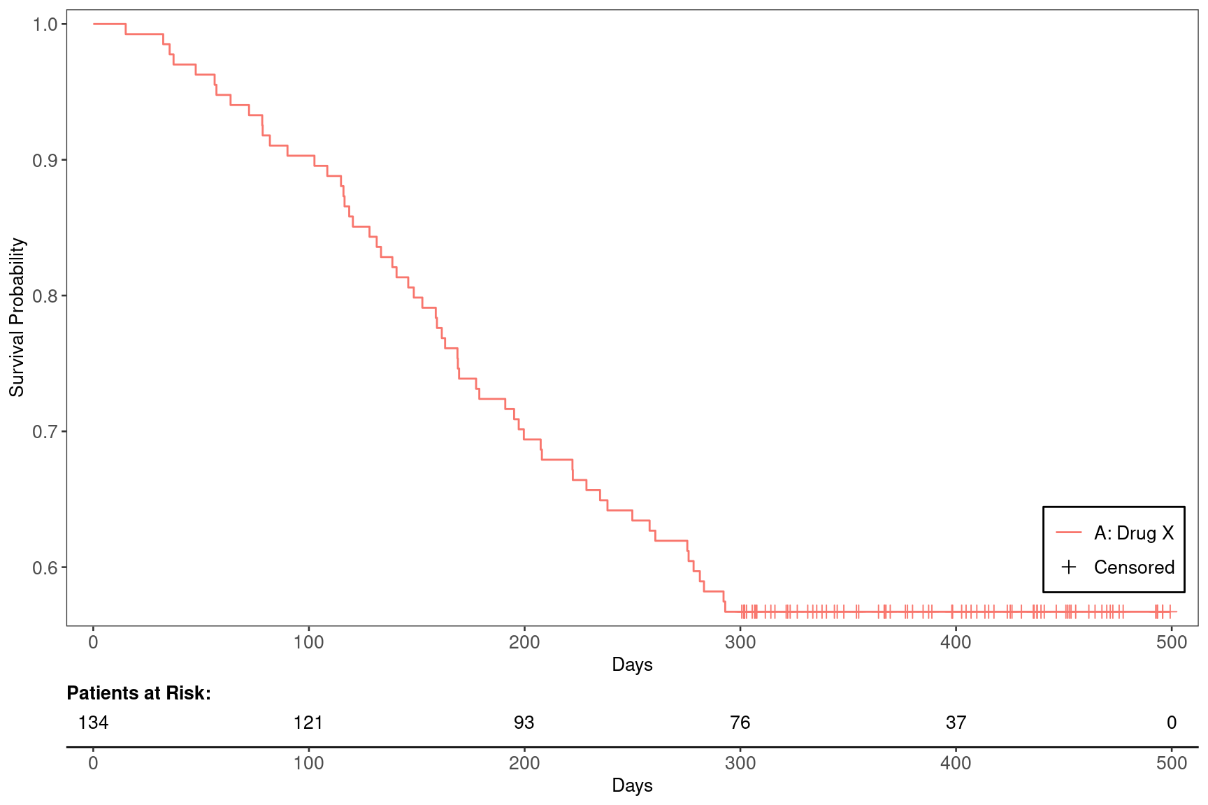
We will use the cadtte data set from the random.cdisc.data package to create the Kaplan-Meier (KM) plots. We start by filtering the time-to-event dataset for the overall survival observations and by one treatment arm (A), creating a new variable for event information, and curating a list of variables required to produce the plot.

library(tern)
library(dplyr)
library(ggplot2)
library(grid)

adtte_arm <- random.cdisc.data::cadtte %>%
  df_explicit_na() %>%
  filter(PARAMCD == "OS", ARM == "A: Drug X") %>%
  mutate(is_event = CNSR == 0)

variables <- list(tte = "AVAL", is_event = "is_event", arm = "ARM")

Plot

We can produce the basic graph using the g_km() function from tern.

g_km(
  df = adtte_arm,
  variables = variables,
  annot_surv_med = FALSE,
  rel_height_plot = 0.85
)

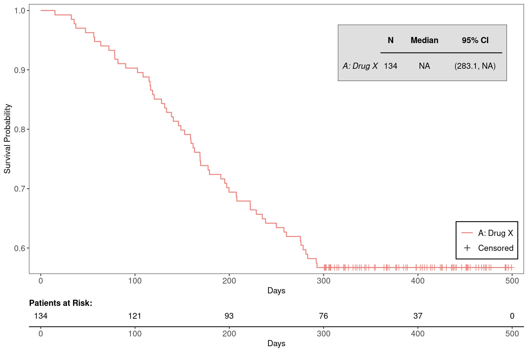
We can also choose to annotate the graph with the median survival time for the overall population using the annot_surv_med = TRUE option.

g_km(
  df = adtte_arm,
  variables = variables,
  annot_surv_med = TRUE,
  rel_height_plot = 0.85
)

Session Info

sessionInfo()

R version 4.4.1 (2024-06-14)
Platform: x86_64-pc-linux-gnu
Running under: Ubuntu 22.04.4 LTS

Matrix products: default
BLAS:   /usr/lib/x86_64-linux-gnu/openblas-pthread/libblas.so.3 
LAPACK: /usr/lib/x86_64-linux-gnu/openblas-pthread/libopenblasp-r0.3.20.so;  LAPACK version 3.10.0

locale:
 [1] LC_CTYPE=en_US.UTF-8       LC_NUMERIC=C              
 [3] LC_TIME=en_US.UTF-8        LC_COLLATE=en_US.UTF-8    
 [5] LC_MONETARY=en_US.UTF-8    LC_MESSAGES=en_US.UTF-8   
 [7] LC_PAPER=en_US.UTF-8       LC_NAME=C                 
 [9] LC_ADDRESS=C               LC_TELEPHONE=C            
[11] LC_MEASUREMENT=en_US.UTF-8 LC_IDENTIFICATION=C       

time zone: Etc/UTC
tzcode source: system (glibc)

attached base packages:
[1] grid      stats     graphics  grDevices utils     datasets  methods  
[8] base     

other attached packages:
[1] ggplot2_3.5.1         dplyr_1.1.4           tern_0.9.5.9022      
[4] rtables_0.6.9.9014    magrittr_2.0.3        formatters_0.5.9.9001

loaded via a namespace (and not attached):
 [1] Matrix_1.7-0                  gtable_0.3.5                 
 [3] jsonlite_1.8.8                compiler_4.4.1               
 [5] tidyselect_1.2.1              stringr_1.5.1                
 [7] tidyr_1.3.1                   splines_4.4.1                
 [9] scales_1.3.0                  yaml_2.3.10                  
[11] fastmap_1.2.0                 lattice_0.22-6               
[13] R6_2.5.1                      labeling_0.4.3               
[15] generics_0.1.3                knitr_1.48                   
[17] forcats_1.0.0                 rbibutils_2.2.16             
[19] htmlwidgets_1.6.4             backports_1.5.0              
[21] checkmate_2.3.2               tibble_3.2.1                 
[23] munsell_0.5.1                 pillar_1.9.0                 
[25] rlang_1.1.4                   utf8_1.2.4                   
[27] broom_1.0.6                   stringi_1.8.4                
[29] xfun_0.47                     cli_3.6.3                    
[31] withr_3.0.1                   Rdpack_2.6.1                 
[33] digest_0.6.37                 cowplot_1.1.3                
[35] lifecycle_1.0.4               vctrs_0.6.5                  
[37] evaluate_0.24.0               glue_1.7.0                   
[39] farver_2.1.2                  codetools_0.2-20             
[41] survival_3.7-0                random.cdisc.data_0.3.15.9009
[43] fansi_1.0.6                   colorspace_2.1-1             
[45] purrr_1.0.2                   rmarkdown_2.28               
[47] tools_4.4.1                   pkgconfig_2.0.3              
[49] htmltools_0.5.8.1