SFG2

Survival Forest Graphs for Overall Population and by Percentiles of Continuous Biomarker

SFG

We prepare the data similarly as in SFG1. In particular we use again the cut_quantile_bins() function, here to obtain quartile bins of the continuous biomarker BMRKR1.

Code

library(tern)
library(dplyr)

BMRKR1_probs <- c(0.25, 0.5, 0.75)

adtte <- random.cdisc.data::cadtte %>%
  df_explicit_na() %>%
  filter(
    PARAMCD == "OS"
  ) %>%
  mutate(
    AVAL = day2month(AVAL),
    AVALU = "Months",
    is_event = CNSR == 0,
    ARM_BIN = fct_collapse_only(
      ARM,
      CTRL = c("B: Placebo"),
      TRT = c("A: Drug X", "C: Combination")
    ),
    BMRKR1 = ifelse(BEP01FL == "N", NA, BMRKR1),
    BMRKR1_BIN = explicit_na(cut_quantile_bins(BMRKR1, BMRKR1_probs)),
    BMRKR2 = fct_explicit_na_if(BMRKR2, BEP01FL == "N")
  ) %>%
  var_relabel(
    BEP01FL = "BEP",
    BMRKR2 = "Biomarker (Categorical)",
    BMRKR1_BIN = "Biomarker (Binned)"
  )

For the calculations, we start by getting the levels from BMRKR1_BIN which saves us typing them manually in the groups_lists definition. This definition is required here so that we can have overlapping subgroups.

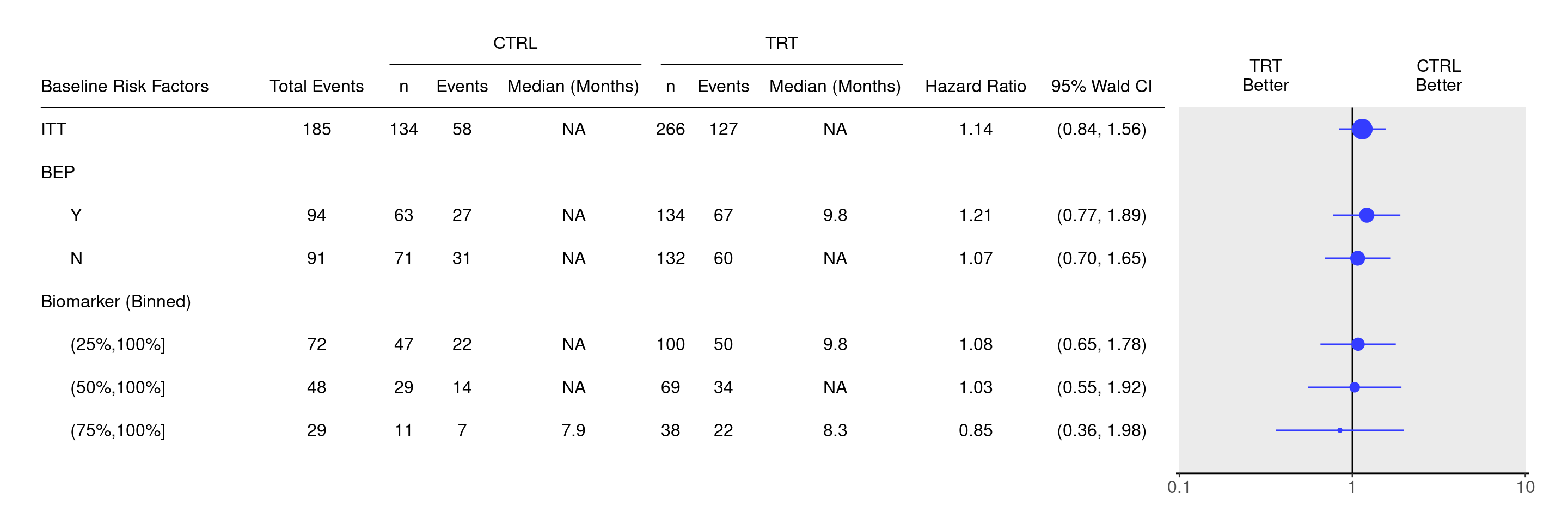
Code

BMRKR1_BIN_levels <- levels(adtte$BMRKR1_BIN)

tbl <- extract_survival_subgroups(
  variables = list(
    tte = "AVAL",
    is_event = "is_event",
    arm = "ARM_BIN",
    subgroups = c("BEP01FL", "BMRKR1_BIN")
  ),
  label_all = "ITT",
  groups_lists = list(
    BMRKR1_BIN = list(
      "(25%,100%]" = BMRKR1_BIN_levels[2:4],
      "(50%,100%]" = BMRKR1_BIN_levels[3:4],
      "(75%,100%]" = BMRKR1_BIN_levels[4]
    )
  ),
  data = adtte
)

result <- basic_table() %>%
  tabulate_survival_subgroups(
    df = tbl,
    vars = c("n_tot_events", "n", "n_events", "median", "hr", "ci"),
    time_unit = adtte$AVALU[1]
  )

We can now produce the forest plot using the g_forest() function from tern based on this result table.

Code

g_forest(result)

Code

sessionInfo()

R version 4.4.1 (2024-06-14)
Platform: x86_64-pc-linux-gnu
Running under: Ubuntu 22.04.4 LTS

Matrix products: default
BLAS:   /usr/lib/x86_64-linux-gnu/openblas-pthread/libblas.so.3 
LAPACK: /usr/lib/x86_64-linux-gnu/openblas-pthread/libopenblasp-r0.3.20.so;  LAPACK version 3.10.0

locale:
 [1] LC_CTYPE=en_US.UTF-8       LC_NUMERIC=C              
 [3] LC_TIME=en_US.UTF-8        LC_COLLATE=en_US.UTF-8    
 [5] LC_MONETARY=en_US.UTF-8    LC_MESSAGES=en_US.UTF-8   
 [7] LC_PAPER=en_US.UTF-8       LC_NAME=C                 
 [9] LC_ADDRESS=C               LC_TELEPHONE=C            
[11] LC_MEASUREMENT=en_US.UTF-8 LC_IDENTIFICATION=C       

time zone: Etc/UTC
tzcode source: system (glibc)

attached base packages:
[1] stats     graphics  grDevices utils     datasets  methods   base     

other attached packages:
[1] dplyr_1.1.4           tern_0.9.5.9022       rtables_0.6.9.9014   
[4] magrittr_2.0.3        formatters_0.5.9.9001

loaded via a namespace (and not attached):
 [1] Matrix_1.7-0                  gtable_0.3.5                 
 [3] jsonlite_1.8.8                compiler_4.4.1               
 [5] tidyselect_1.2.1              stringr_1.5.1                
 [7] tidyr_1.3.1                   splines_4.4.1                
 [9] scales_1.3.0                  yaml_2.3.10                  
[11] fastmap_1.2.0                 lattice_0.22-6               
[13] ggplot2_3.5.1                 R6_2.5.1                     
[15] labeling_0.4.3                generics_0.1.3               
[17] knitr_1.48                    forcats_1.0.0                
[19] rbibutils_2.2.16              htmlwidgets_1.6.4            
[21] backports_1.5.0               checkmate_2.3.2              
[23] tibble_3.2.1                  munsell_0.5.1                
[25] pillar_1.9.0                  rlang_1.1.4                  
[27] utf8_1.2.4                    broom_1.0.6                  
[29] stringi_1.8.4                 xfun_0.47                    
[31] cli_3.6.3                     withr_3.0.1                  
[33] Rdpack_2.6.1                  digest_0.6.37                
[35] grid_4.4.1                    cowplot_1.1.3                
[37] lifecycle_1.0.4               vctrs_0.6.5                  
[39] evaluate_0.24.0               glue_1.7.0                   
[41] farver_2.1.2                  codetools_0.2-20             
[43] survival_3.7-0                random.cdisc.data_0.3.15.9009
[45] fansi_1.0.6                   colorspace_2.1-1             
[47] purrr_1.0.2                   rmarkdown_2.28               
[49] tools_4.4.1                   pkgconfig_2.0.3              
[51] htmltools_0.5.8.1

Reuse