SFG6C

Survival Forest Graph for Multiple Continuous Biomarkers with Stratification

---

Setup

These templates are helpful when we are interested in modelling the effects of continuous biomarker variables on a time-to-event (survival) outcome, conditional on covariates and/or stratification variables included in Cox proportional hazards regression models. We would like to assess how the estimates effects change when we look at different subgroups.

In detail the differences to the other survival forest graphs (SFG1 to SFG5) are the following:

• The extract_survival_subgroups() and tabulate_survival_subgroups() functions evaluate the treatment effects comparing two arms, across subgroups. On the other hand, the extract_survival_biomarkers() and tabulate_survival_biomarkers() functions used here in SFG6 evaluate the effects from continuous biomarkers in the Cox proportional hazards models, across subgroups.
• The extract_survival_subgroups() and tabulate_survival_subgroups() functions only allow specification of a single treatment arm variable, while the extract_survival_biomarkers() and tabulate_survival_biomarkers() allow to look at multiple continuous biomarker variables at once.
• In addition to the treatment arms, the use of extract_survival_subgroups() and tabulate_survival_subgroups() functions can be extended to other binary variables, as done in SFG3 and SFG4. For example, we could define the binarized ARM variable as AGE>=65 vs. AGE<65 and then look at the odds ratios across subgroups. For the extract_survival_biomarkers() and tabulate_survival_biomarkers() functions, we could use the original continuous biomarker variable AGE, and then look at the estimated effect across subgroups.

Similarly like in SFG3, we will use the cadtte data set from the random.cdisc.data package. Here we just filter for the overall survival outcome in a single arm in the biomarker evaluable population.

library(tern)
library(dplyr)

adtte_f <- random.cdisc.data::cadtte %>%
  df_explicit_na() %>%
  filter(
    PARAMCD == "OS",
    ARM == "A: Drug X",
    BEP01FL == "Y"
  ) %>%
  mutate(
    AVAL = day2month(AVAL),
    AVALU = "Months",
    is_event = CNSR == 0
  ) %>%
  var_relabel(
    BEP01FL = "BEP",
    BMRKR1 = "Biomarker (Countinuous)"
  )

Plot

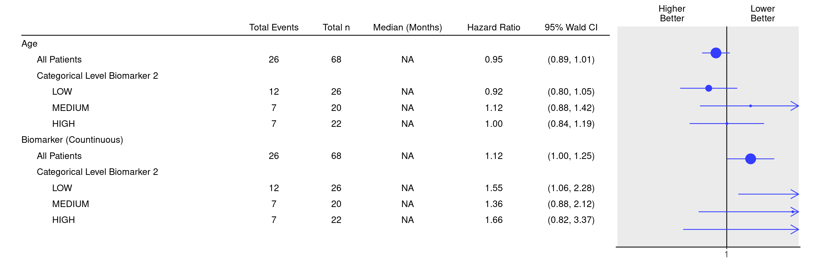
Finally we can also specify stratification variables with the strata variable element, then the corresponding variables are used for stratification in the Cox proportional hazards models.

df <- extract_survival_biomarkers(
  variables = list(
    tte = "AVAL",
    is_event = "is_event",
    biomarkers = c("BMRKR1", "AGE"),
    covariates = "SEX",
    subgroups = "BMRKR2",
    strata = c("STRATA1", "STRATA2")
  ),
  data = adtte_f
)

result <- tabulate_survival_biomarkers(
  df = df,
  vars = c("n_tot_events", "n_tot", "median", "hr", "ci"),
  time_unit = adtte_f$AVALU[1]
)
g_forest(result, xlim = c(0.6, 1.4))

Note that warnings might be issued if the model contains e.g. too few events in the resulting strata, in that case you might want to reduce the number of stratification variables.

Session Info

sessionInfo()

R version 4.4.1 (2024-06-14)
Platform: x86_64-pc-linux-gnu
Running under: Ubuntu 22.04.4 LTS

Matrix products: default
BLAS:   /usr/lib/x86_64-linux-gnu/openblas-pthread/libblas.so.3 
LAPACK: /usr/lib/x86_64-linux-gnu/openblas-pthread/libopenblasp-r0.3.20.so;  LAPACK version 3.10.0

locale:
 [1] LC_CTYPE=en_US.UTF-8       LC_NUMERIC=C              
 [3] LC_TIME=en_US.UTF-8        LC_COLLATE=en_US.UTF-8    
 [5] LC_MONETARY=en_US.UTF-8    LC_MESSAGES=en_US.UTF-8   
 [7] LC_PAPER=en_US.UTF-8       LC_NAME=C                 
 [9] LC_ADDRESS=C               LC_TELEPHONE=C            
[11] LC_MEASUREMENT=en_US.UTF-8 LC_IDENTIFICATION=C       

time zone: Etc/UTC
tzcode source: system (glibc)

attached base packages:
[1] stats     graphics  grDevices utils     datasets  methods   base     

other attached packages:
[1] dplyr_1.1.4           tern_0.9.5.9022       rtables_0.6.9.9014   
[4] magrittr_2.0.3        formatters_0.5.9.9001

loaded via a namespace (and not attached):
 [1] utf8_1.2.4                    generics_0.1.3               
 [3] tidyr_1.3.1                   stringi_1.8.4                
 [5] lattice_0.22-6                digest_0.6.37                
 [7] evaluate_0.24.0               grid_4.4.1                   
 [9] fastmap_1.2.0                 jsonlite_1.8.8               
[11] Matrix_1.7-0                  backports_1.5.0              
[13] survival_3.7-0                purrr_1.0.2                  
[15] fansi_1.0.6                   scales_1.3.0                 
[17] codetools_0.2-20              abind_1.4-8                  
[19] Rdpack_2.6.1                  cli_3.6.3                    
[21] rlang_1.1.4                   rbibutils_2.2.16             
[23] cowplot_1.1.3                 munsell_0.5.1                
[25] splines_4.4.1                 withr_3.0.1                  
[27] yaml_2.3.10                   tools_4.4.1                  
[29] checkmate_2.3.2               colorspace_2.1-1             
[31] ggplot2_3.5.1                 forcats_1.0.0                
[33] broom_1.0.6                   vctrs_0.6.5                  
[35] R6_2.5.1                      lifecycle_1.0.4              
[37] stringr_1.5.1                 car_3.1-2                    
[39] htmlwidgets_1.6.4             pkgconfig_2.0.3              
[41] pillar_1.9.0                  gtable_0.3.5                 
[43] glue_1.7.0                    xfun_0.47                    
[45] tibble_3.2.1                  tidyselect_1.2.1             
[47] knitr_1.48                    farver_2.1.2                 
[49] htmltools_0.5.8.1             labeling_0.4.3               
[51] rmarkdown_2.28                carData_3.0-5                
[53] random.cdisc.data_0.3.15.9009 compiler_4.4.1