SFG2D

Survival Forest Graph for Overall Population and by Intervals of Continuous Biomarker with “Greater Than a Numerical Cutoff”

SFG

We prepare the data similarly as in SFG1. In particular we use again the cut_quantile_bins() function, here to obtain quartile bins of the continuous biomarker BMRKR1.

Code

library(tern)
library(dplyr)

BMRKR1_probs <- c(0.25, 0.5, 0.75)

adtte <- random.cdisc.data::cadtte %>%
  df_explicit_na() %>%
  filter(
    PARAMCD == "OS"
  ) %>%
  mutate(
    AVAL = day2month(AVAL),
    AVALU = "Months",
    is_event = CNSR == 0,
    ARM_BIN = fct_collapse_only(
      ARM,
      CTRL = c("B: Placebo"),
      TRT = c("A: Drug X", "C: Combination")
    ),
    BMRKR1 = ifelse(BEP01FL == "N", NA, BMRKR1),
    BMRKR1_BIN = explicit_na(cut_quantile_bins(BMRKR1, BMRKR1_probs)),
    BMRKR2 = fct_explicit_na_if(BMRKR2, BEP01FL == "N")
  ) %>%
  var_relabel(
    BEP01FL = "BEP",
    BMRKR2 = "Biomarker (Categorical)",
    BMRKR1_BIN = "Biomarker (Binned)"
  )

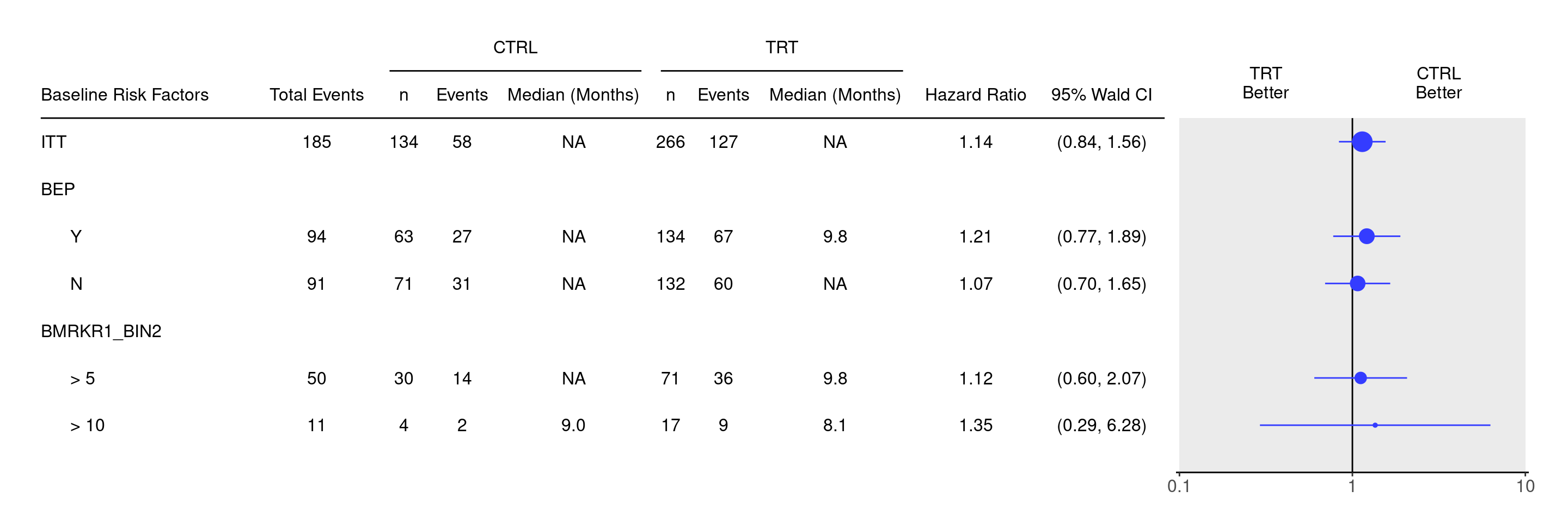
We start by deriving a new biomarker variable BMRKR1_BIN2 with greater than numerical cutoffs for BMRKR1 using the cut() funciton, and then tabulate the statistics as above to be able to use them as an input for the forest plot.

Code

BMRKR1_cuts <- c(0, 5, 10, Inf)

adtte <- adtte %>%
  mutate(
    BMRKR1_BIN2 = explicit_na(cut(
      BMRKR1,
      BMRKR1_cuts,
      include.lowest = FALSE,
      right = FALSE
    ))
  )

tbl <- extract_survival_subgroups(
  variables = list(
    tte = "AVAL",
    is_event = "is_event",
    arm = "ARM_BIN",
    subgroups = c("BEP01FL", "BMRKR1_BIN2")
  ),
  label_all = "ITT",
  groups_lists = list(
    BMRKR1_BIN2 = list(
      "> 5" = c("[5,10)", "[10,Inf)"),
      "> 10" = "[10,Inf)"
    )
  ),
  data = adtte
)

result <- basic_table() %>%
  tabulate_survival_subgroups(
    df = tbl,
    vars = c("n_tot_events", "n", "n_events", "median", "hr", "ci"),
    time_unit = adtte$AVALU[1]
  )

We can now produce forest plot using g_forest() function from tern based on this result table.

Code

g_forest(result)

Code

sessionInfo()

R version 4.4.1 (2024-06-14)
Platform: x86_64-pc-linux-gnu
Running under: Ubuntu 22.04.4 LTS

Matrix products: default
BLAS:   /usr/lib/x86_64-linux-gnu/openblas-pthread/libblas.so.3 
LAPACK: /usr/lib/x86_64-linux-gnu/openblas-pthread/libopenblasp-r0.3.20.so;  LAPACK version 3.10.0

locale:
 [1] LC_CTYPE=en_US.UTF-8       LC_NUMERIC=C              
 [3] LC_TIME=en_US.UTF-8        LC_COLLATE=en_US.UTF-8    
 [5] LC_MONETARY=en_US.UTF-8    LC_MESSAGES=en_US.UTF-8   
 [7] LC_PAPER=en_US.UTF-8       LC_NAME=C                 
 [9] LC_ADDRESS=C               LC_TELEPHONE=C            
[11] LC_MEASUREMENT=en_US.UTF-8 LC_IDENTIFICATION=C       

time zone: Etc/UTC
tzcode source: system (glibc)

attached base packages:
[1] stats     graphics  grDevices utils     datasets  methods   base     

other attached packages:
[1] dplyr_1.1.4           tern_0.9.5.9022       rtables_0.6.9.9014   
[4] magrittr_2.0.3        formatters_0.5.9.9001

loaded via a namespace (and not attached):
 [1] Matrix_1.7-0                  gtable_0.3.5                 
 [3] jsonlite_1.8.8                compiler_4.4.1               
 [5] tidyselect_1.2.1              stringr_1.5.1                
 [7] tidyr_1.3.1                   splines_4.4.1                
 [9] scales_1.3.0                  yaml_2.3.10                  
[11] fastmap_1.2.0                 lattice_0.22-6               
[13] ggplot2_3.5.1                 R6_2.5.1                     
[15] labeling_0.4.3                generics_0.1.3               
[17] knitr_1.48                    forcats_1.0.0                
[19] rbibutils_2.2.16              htmlwidgets_1.6.4            
[21] backports_1.5.0               checkmate_2.3.2              
[23] tibble_3.2.1                  munsell_0.5.1                
[25] pillar_1.9.0                  rlang_1.1.4                  
[27] utf8_1.2.4                    broom_1.0.6                  
[29] stringi_1.8.4                 xfun_0.47                    
[31] cli_3.6.3                     withr_3.0.1                  
[33] Rdpack_2.6.1                  digest_0.6.37                
[35] grid_4.4.1                    cowplot_1.1.3                
[37] lifecycle_1.0.4               vctrs_0.6.5                  
[39] evaluate_0.24.0               glue_1.7.0                   
[41] farver_2.1.2                  codetools_0.2-20             
[43] survival_3.7-0                random.cdisc.data_0.3.15.9009
[45] fansi_1.0.6                   colorspace_2.1-1             
[47] purrr_1.0.2                   rmarkdown_2.28               
[49] tools_4.4.1                   pkgconfig_2.0.3              
[51] htmltools_0.5.8.1

Reuse