Correlation between PFS and OS

Here we describe how the correlation between progression-free survival (PFS) and overall survival (OS) is computed.

Introduction

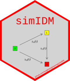
The illness-death model used in simIDM is designed to jointly model PFS and OS as endpoints in an oncology clinical trial. Within each treatment arm, the model is specified through the transition hazards \(\lambda_{01}(t)\), \(\lambda_{02}(t)\) and \(\lambda_{12}(t)\). This approach allows us to consider the joint distribution of the two endpoints and to derive the correlation between PFS and OS directly from the assumed transition hazards.

Cor(PFS, OS): Statistical Background

Meller, Beyersmann, and Rufibach (2019) derive a closed formula for \(Cor(PFS,OS)\). The general formula for the correlation is \[ Cor(PFS, OS) = \frac{Cov(PFS, OS)}{\sqrt{Var(PFS) \, Var(OS)}}. \] The expected values of PFS and OS can be derived via the survival functions for PFS and OS, respectively: \[ \mathbb{E}(PFS) = \int_{0}^{\infty} S_{PFS}(u) \,du \] and \[ \mathbb{E}(OS) = \int_{0}^{\infty} S_{OS}(u) \,du. \] The variance of PFS and OS are computed as follows: \[ Var(PFS) = \mathbb{E}(PFS^2) - \mathbb{E}(PFS)^2 \] where \[ \mathbb{E}(PFS^2) = 2 \cdot\int_{0}^{\infty} u \cdot S_{PFS}(u) \,du \] and in a similar way for \(Var(OS)\). \(Cov(PFS,OS)\) is derived using \[ Cov(PFS,OS) = \mathbb{E}(PFS \cdot OS) - \mathbb{E}(PFS) \cdot \mathbb{E}(OS) \] together with the general formula for deriving expected survival times, and where \[ P(PFS \cdot OS > t) = P(PFS > \sqrt{t}) \, + \int_{\left(0, \sqrt{t} \right]} P_{11}(u,t/u;u) \cdot P(PFS>u-) \cdot \lambda_{01}(u) \, du. \] This requires the transition probability \(P_{11}(s,t;t_{1})\), which has the form of a standard survival function: \[ P_{11}(s,t;t_{1}) = exp \left( -\int_{s}^{t} \lambda_{12}(u;t_{1}) \, du\right). \]

We can compute the correlation based on assumptions or estimate it from data. Both work by simply plugging in assumed or estimated survival functions.

Example: Computing Cor(PFS, OS) directly

We consider three alternative scenarios to model transition hazards within a treatment arm:

constant (exponential distribution)
Weibull
piecewise constant

library(simIDM)

# constant hazards:
transitionExp <- exponential_transition(h01 = 1.2, h02 = 1.5, h12 = 1.6)

# Weibull hazards:
transitionWeib <- weibull_transition(h01 = 1, h02 = 1.2, h12 = 1.3, p01 = 1.1, p02 = 0.8, p12 = 1.2)

# piecewise constant hazards:
transitionPwc <- piecewise_exponential(
  h01 = c(1, 1.3), h02 = c(0.8, 1.5), h12 = c(1, 1),
  pw01 = c(0, 3), pw02 = c(0, 1), pw12 = c(0, 8)
)

Now, we can compute the PFS-OS correlation with corTrans():

# constant hazards:
corTrans(transitionExp)
#> [1] 0.580381

# Weibull hazards:
corTrans(transitionWeib)
#> [1] 0.7024952

# piecewise constant hazards:
corTrans(transitionPwc)
#> [1] 0.4464817

Estimating Cor(PFS, OS) from data

In case we are given trial data and want to estimate the PFS-OS correlation from the data, the following approach can be adopted:

Specify the assumed distribution family.
Estimate the transition hazards under this assumption from the data.
Compute the correlation of PFS and OS.

We can estimate the parameters via maximum likelihood (ML), using the log-likelihood based on the counting process notation of Andersen et al. (1993), see also Meller, Beyersmann, and Rufibach (2019): \[ L(\theta) = \sum_{i=1}^{n} \sum_{k=1}^{3} \left( \log \left[ \lambda_{k}(t_{ik})^{d_{ik}} \frac{S_{k}(t_{ik})}{S_{k}(t_{0ik})} \right] \times \mathbb{I}(i \in Y_{ik}) \right), \] where the sum is over all \(n\) individuals. \(k \in \{ 1, 2, 3 \}\) is a simplified notation for the transitions 0 \(\rightarrow\) 1, 0 \(\rightarrow\) 2 and 1 \(\rightarrow\) 2, \(\lambda_{k}\) is the corresponding transition hazard and \(S_{k}\) the survival function. \(d_{ik}\) is an indicator function, taking the value 1 if the \(i\)-th individual made the \(k\)-th transition and \(t_{0ik}\) and \(t_{ik}\) are the time the \(i\)-th individual enters and exits, respectively, the root state of the \(k\)-th transition. The indicator function at the end of the formula is equal to 1 if the \(i\)-th individual is at risk for the transition \(k\) and 0 otherwise.

Example: Estimating Cor(PFS, OS) from data

Currently, this package supports parameter estimation for assuming either constant or Weibull transition hazards. The estimateParams() function expects a data argument of the same format as used throughout the package, and a transition argument of class TransitionParameters, specifying the assumed distribution and desired starting values for ML estimation. To demonstrate this, we simulate data using constant transition hazards:

transitionExp <- exponential_transition(h01 = 1.2, h02 = 1.5, h12 = 1.6)
simData <- getOneClinicalTrial(
  nPat = c(500), transitionByArm = list(transitionExp),
  dropout = list(rate = 0.8, time = 12),
  accrual = list(param = "time", value = 1)
)

We can estimate the parameters as follows:

# Create TransitionParameters object with starting values for ML estimation:
transition <- exponential_transition(h01 = 1, h02 = 1, h12 = 1)
# Estimate parameters:
est <- estimateParams(data = simData, transition = transition)
# Get estimated transition hazards:
est$hazards
#> $h01
#> [1] 1.10497
#> 
#> $h02
#> [1] 1.355154
#> 
#> $h12
#> [1] 1.705242

Then, in a final step, we pass est to corTrans() to compute the PFS-OS correlation.

Alternatively, one can combine these steps efficiently via corPFSOS(), which has an additional bootstrap argument to quantify the uncertainty of the correlation estimate:

corPFSOS(data = simData, transition = transition, bootstrap = TRUE, conf_level = 0.95)
#> $corPFSOS
#> [1] 0.6389041
#> 
#> $lower
#>      2.5% 
#> 0.5803577 
#> 
#> $upper
#>    97.5% 
#> 0.837497

References

Andersen, Per Kragh, Ørnulf Borgan, Richard D Gill, and Niels Keiding. 1993. “Statistical Models Based on Counting Processes.” Springer Series in Statistics.