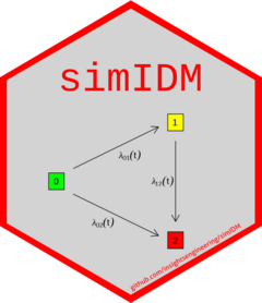
Survival multistate models are a powerful and flexible tool for modeling and analyzing complex time-to-event data. The three-state illness-death model can be used to jointly model the oncology endpoints progression-free survival (PFS) and overall survival (OS). Jointly modeling the endpoints PFS and OS with the illness-death model has the major advantage of both adequately accounting for the correlation of the two endpoints and eliminating the need of the strong assumption of proportional hazards. This package provides the tools to simulate a large number of clinical trials with endpoints OS and PFS based on the illness-death model, which can be used for trail planning, for example. The simulation set-up allows random and event-driven censoring, an arbitrary number of treatment arms, staggered study entry and drop-out. Exponentially, Weibull and piecewise exponentially distributed survival times can be generated. In addition, the correlation between PFS and OS can be calculated based on the simulation scenario, or estimated from a given data set.
Scope:
- Simulation of the illness-death model with constant, Weibull or piecewise constant transition hazards.
- Conversion of the transition times to PFS and OS survival times.
- Correlation between PFS and OS survival times can be calculated.
Main Features:
- Exponentially, Weibull and piecewise exponentially distributed survival times.
- Random censoring and event-driven censoring after a pre-specified number of PFS or OS events.
- Arbitrary number of treatment arms and flexible randomization ratio.
- Staggered study entry.
- Derivation of PFS and OS survival functions from transition hazards.
- Correlation between PFS and OS can be estimated from a given data set.
Installation
Development
You can install the current development version from GitHub with:
if (!require("remotes")) {
  install.packages("remotes")
}
remotes::install_github("insightsengineering/simIDM")
Getting Started
See also the quick start vignette or get started by trying out this example:
library(simIDM)
transitionGroup1 <- exponential_transition(h01 = 1.2, h02 = 1.5, h12 = 1.6)
transitionGroup2 <- exponential_transition(h01 = 1, h02 = 1.3, h12 = 1.7)

simStudies <- getClinicalTrials(
  nRep = 100, nPat = c(50, 50), seed = 1234, datType = "1rowPatient",
  transitionByArm = list(transitionGroup1, transitionGroup2), dropout = list(rate = 0.1, time = 12),
  accrual = list(param = "intensity", value = 12)
)
We get as output a list with nRep elements, each containing a data set of a single simulated trial.
head(simStudies[[1]])
#>   id trt    PFStime CensoredPFS PFSevent    OStime CensoredOS OSevent
#> 1  1   1 0.08087899           0        1 2.0330026          0       1
#> 2  2   1 0.84758881           0        1 0.8475888          0       1
#> 3  3   1 0.18276912           0        1 0.1968048          0       1
#> 4  4   1 0.13789870           0        1 1.2899802          0       1
#> 5  5   1 0.06458797           0        1 0.6901351          0       1
#> 6  6   1 0.83894555           0        1 1.0709457          0       1
#>   recruitTime OStimeCal PFStimeCal
#> 1   0.8516769  2.884679  0.9325558
#> 2   4.1068045  4.954393  4.9543933
#> 3   2.3596282  2.556433  2.5423973
#> 4   1.1682298  2.458210  1.3061285
#> 5   0.7710655  1.461201  0.8356535
#> 6   3.1585892  4.229535  3.9975347
Citing simIDM
To cite simIDM please see here.
