simIDM: Power and Type I Error Calculations
Alexandra Erdmann
11/14/2022
Source:vignettes/trialplanning.Rmd
trialplanning.RmdIntroduction
The goal of this vignette is to show with a simple example how the
package can be used for planning a study design. Jointly modeling the
endpoints PFS and OS with the illness-death model has the major
advantage that, on the one hand, the correlation of the two endpoints is
taken into account properly and, on the other hand, the strong
assumption of proportional hazards is not required. OS is defined as the
time to reach the absorbing state death, and PFS is defined as the time
to reach the absorbing state death or the intermediate
state progression, whichever occurs first. Figure 1 shows
the multistate model with the corresponding transition hazards. In the
vignette, we show how type-I errors and statistical power can be
estimated from simulations and give an idea on how this can be used to
plan complex study trials, in which PFS and OS both play a relevant
role.

Figure 1 - Multistate model with indermediate state progession and absorbing state death
Scenario - PFS and OS as co-primary endpoints
We consider the following study design:
- PFS and OS as co-primary endpoints with one final analysis each
- treatment vs control group, 1:1 randomization ratio (but note that in principle any randomization ratio can be implemented)
- global significance level: 5 %
- the standard log-rank test used to detect a significant difference between the groups
- statistical power to detect a difference between the groups should be 80 % for each endpoint
- 5 % drop-out rate within 12 time units
- accrual of 100 patients per time unit
Using the multistate model approach implies that the trial planning is based on assumptions on the transition hazards in each arm, i.e. six hazards in total (which induces assumptions on the endpoints PFS and OS). In our example scenario, we assume constant transition hazards and a small effect of the treatment on hazards from the initial state to death. Median time until PFS in the control arm is 0.99 time units, in the treatment arm 1.44 time units. The median time until an OS event in the control group is 1.94 time units, in the treatment group 2.29 time units. Figure 2 shows the transition hazards, survival functions and the hazard ratios for both endpoints.
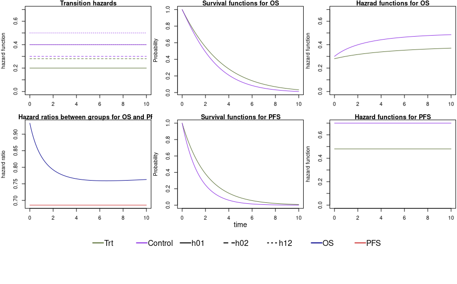
Figure 2 - Transition hazards, survival functions and hazard ratios for our scenario.
The transition hazards are specified as follows:
library(simIDM)
library(survival)
transitionTrt <- exponential_transition(h01 = 0.2, h02 = 0.28, h12 = 0.4)
transitionPl <- exponential_transition(h01 = 0.4, h02 = 0.3, h12 = 0.5)

transitionList <- list(transitionPl, transitionTrt)
The package provides functions that return the values of the PFS or OS survival functions for given transition hazards and time points.
timepoints <- c(0, 0.1, 0.2, 0.3, 0.7, 1, 5)
ExpSurvOS(timepoints, h01 = 0.2, h02 = 0.4, h12 = 0.1)
#> [1] 1.0000000 0.9610787 0.9242317 0.8893403 0.7671856 0.6912219 0.2724845
WeibSurvOS(timepoints, h01 = 0.2, h02 = 0.5, h12 = 2.1, p01 = 1.2, p02 = 0.9, p12 = 1)
#> [1] 1.00000000 0.93822237 0.88590654 0.83706584 0.66353707 0.55296798 0.03684786
PWCsurvOS(timepoints,
  h01 = c(0.3, 0.5), h02 = c(0.5, 0.8), h12 = c(0.7, 1),
  pw01 = c(0, 4), pw02 = c(0, 8), pw12 = c(0, 3)
)
#> [1] 1.00000000 0.95094877 0.90378713 0.85849702 0.69546105 0.59109798 0.03945673
There are also functions for PFS survival functions available. ## Type-I error - simulation under \(H_0\)
For the simulation under \(H_0\) we
set the transition hazards for the treatment group equal to the control
group. Then, we use our function getClinicalTrials() to
generate a large number of simulated trials. For this example we use 100
iterations, however for applications we would recommend a higher number,
e.g. 10000
transitionListNULL <- list(transitionPl, transitionPl)
nRep <- 100
SimNULL <- getClinicalTrials(
  nRep = nRep, nPat = c(800, 800), seed = 1238, datType = "1rowPatient",
  transitionByArm = transitionListNULL,
  dropout = list(rate = 0.05, time = 12), accrual = list(param = "intensity", value = 100)
)
The simulation can be used to determine critical values for the log-rank test for both endpoints, such that the global significance level is controlled at 5%. As a starting point we use the critical values, such that the two-sided log-rank test has a significance level of 4 % for the OS endpoint and 1% for the PFS endpoint, i.e. we simply split the global significance level. This is a common approach for trials with co-primary endpoints.
alphaOS <- 0.04
alphaPFS <- 0.01
CriticalOS <- abs(qnorm(alphaOS / 2))
CriticalPFS <- abs(qnorm(alphaPFS / 2))
Using the Schoenfeld approximation, a preliminary sample size
calculation could be made to get an idea of how many events are needed
for 80 % power. For PFS the hazard ratio is known by specification (=
0.6857), for OS an averaged HR can be calculated, e.g. by using the R
package coxphw (Dunkler et al.
2018):
library(coxphw)
avergHR <- function(data) {
  fit <- coxphw(formula = Surv(OStime + 0.001, OSevent) ~ trt, data = data, template = "AHR")
  exp(coef(fit))
}

StudyforAvg <- getClinicalTrials(
  nRep = 100, nPat = c(800, 800), seed = 1238, datType = "1rowPatient",
  transitionByArm = transitionList,
  dropout = list(rate = 0.05, time = 12), accrual = list(param = "intensity", value = 25)
)

averageHR <- sapply(StudyforAvg, avergHR)
MeanAverageHR <- mean(averageHR)
In our example, we get an average OS HR of 0.826. We use the standard log-rank test to test difference between groups:
LogRankTest <- function(data, endpoint, critical) {
  time <- if (endpoint == "OS") {
    data$OStime
  } else if (endpoint == "PFS") {
    data$PFStime
  }
  event <- if (endpoint == "OS") {
    data$OSevent
  } else if (endpoint == "PFS") {
    data$PFSevent
  }
  LogRank <- survdiff(Surv(time, event) ~ trt, data)
  Passed <- sqrt(LogRank$chisq) > critical
  return(Passed)
}
and apply it to PFS and OS in our simulated trials.
# Step 1: cut simulated data at time-point of OS/PFS analysis
studyAtPFSAna <- lapply(SimNULL, censoringByNumberEvents,
  eventNum = 329, typeEvent = "PFS"
)

studyAtOSAna <- lapply(SimNULL, censoringByNumberEvents,
  eventNum = 660, typeEvent = "OS"
)

# Step 2: get results of log-rank test for both endpoints and all studies

TestPassedPFS <- lapply(studyAtPFSAna, LogRankTest, endpoint = "PFS", CriticalPFS)
TestPassedOS <- lapply(studyAtOSAna, LogRankTest, endpoint = "OS", CriticalOS)
We estimate the type-I error for each endpoint and the global type-I error by counting the significant tests under \(H_0\). The global type-I error is empirically estimated by counting the trials in which either a significant log-rank test is observed for the PFS endpoint or for the OS endpoint.
# empirical type-I error of PFS
empAlphaPFS <- 100 * (sum(unlist(TestPassedPFS)) / nRep)

# empirical type-I error of OS
empAlphaOS <- 100 * (sum(unlist(TestPassedOS)) / nRep)

TestBoth <- (unlist(TestPassedPFS) + unlist(TestPassedOS) >= 1)
# empirical global significance level
empGlobalAlpha <- 100 * (sum(TestBoth) / nRep)
In this example, the empirical significance level is close to 5%. If the empirical type-I error is lower or higher than 5%, the critical values used for the log-rank test can be adjusted until a significance level close to 5% is obtained. This could be done, for example, in the following way:
while (empGlobalAlpha < 4.9) {
  CriticalOS <- CriticalOS - 0.01
  CriticalPFS <- CriticalPFS - 0.01

  TestPassedPFS <- lapply(studyAtPFSAna, LogRankTest, endpoint = "PFS", CriticalPFS)
  TestPassedOS <- lapply(studyAtOSAna, LogRankTest, endpoint = "OS", CriticalOS)
  TestBoth <- (unlist(TestPassedPFS) + unlist(TestPassedOS) >= 1)

  # empirical global significance level
  empGlobalAlpha <- 100 * (sum(TestBoth) / nRep)
}
Sample size and power calculation - simulation under \(H_1\)
Next, we simulate a large number of trials under \(H_1\) to get the empirical power.
SimH1 <- getClinicalTrials(
  nRep = nRep, nPat = c(800, 800), seed = 1238, datType = "1rowPatient",
  transitionByArm = transitionList,
  dropout = list(rate = 0.05, time = 12), accrual = list(param = "intensity", value = 100)
)
We derive the empirical power by counting the significant log-rank tests under \(H_1\) for each endpoint. The multistate model approach allows us to easily estimate further interesting metrics, that affect both endpoints. For example, the joint power, i.e. the power that both endpoints in one trial are significant, if each endpoint is analyzed at its planned time-point.
# Step 1: cut simulated data at time-point of OS/PFS analysis
studyAtPFSAnaH1 <- lapply(SimH1, censoringByNumberEvents,
  eventNum = 329, typeEvent = "PFS"
)

studyAtOSAnaH1 <- lapply(SimH1, censoringByNumberEvents,
  eventNum = 660, typeEvent = "OS"
)

# Step 2: get results of log-rank test for both endpoints and all studies.

logrankPFSH1 <- lapply(studyAtPFSAnaH1, LogRankTest,
  endpoint = "PFS", CriticalPFS
)
logrankOSH1 <- lapply(studyAtOSAnaH1, LogRankTest,
  endpoint = "OS", CriticalOS
)

TestPassedPFSH1 <- lapply(logrankPFSH1, `[[`, 1)
TestPassedOSH1 <- lapply(logrankOSH1, `[[`, 1)
# Step 3: count significant log-rank tests.
# empirical power PFS
empPowerPFS <- 100 * (sum(unlist(TestPassedPFSH1)) / nRep)
empPowerPFS
#> [1] 79
# empirical power OS
empPowerOS <- 100 * (sum(unlist(TestPassedOSH1)) / nRep)
empPowerOS
#> [1] 64
# joint power
TestBothH1 <- (unlist(TestPassedPFSH1) + unlist(TestPassedOSH1) == 2)

jointPower <- 100 * (sum(TestBothH1) / nRep)
jointPower
#> [1] 54
For the endpoint OS, the number of events has to be increased to obtain a power of 80 %.
It is also possible to derive the median time at which a certain number of events are expected to occur and how many events of the second endpoint have occurred at that time.
# median time
TimePointsPFS <- lapply(SimH1, getTimePoint,
  eventNum = 329, typeEvent = "PFS",
  byArm = FALSE
)
median_timePFS <- median(unlist(TimePointsPFS))

TimePointsOS <- lapply(SimH1, getTimePoint,
  eventNum = 684, typeEvent = "OS",
  byArm = FALSE
)
median_timeOS <- median(unlist(TimePointsOS))

median_timePFS
#> [1] 3.081201
median_timeOS
#> [1] 5.998852

# number of PFS events at time of OS analysis
eventsPFS <- lapply(
  seq_along(TimePointsPFS),
  function(t) {
    return(sum(SimH1[[t]]$OSevent[(SimH1[[t]]$OStime + SimH1[[t]]$recruitTime)
    <= TimePointsPFS[[t]]]))
  }
)
# number of OS events at time of PFS analysis
eventsOS <- lapply(
  seq_along(TimePointsOS),
  function(t) {
    return(sum(SimH1[[t]]$PFSevent[(SimH1[[t]]$PFStime + SimH1[[t]]$recruitTime)
    <= TimePointsOS[[t]]]))
  }
)

nPFS <- mean(unlist(eventsPFS))
nOS <- mean(unlist(eventsOS))

nPFS
#> [1] 225.97
nOS
#> [1] 860.45