Creates a standard Pharmacokinetic (PK) concentration-time profile plot.
This function wraps ggplot2 calls to consistently format PK profiles,
handling log transformations, various summary statistics, and variability measures.
Arguments
- data
(
data.frame)
The dataset containing PK data.- time_var
(
tidy-select)
The time variable (x-axis).- analyte_var
(
tidy-select)
The concentration/analyte variable (y-axis).- group
(
tidy-select)
The grouping/treatment variable.- stat
(
string)
Primary summary statistic:"mean"or"median". Default is"mean".- variability
(
string)
Variability measure:"sd","se","ci","iqr", or"none". Default is"sd".- conf_level
(
numeric)
Confidence level for error bars whenvariability = "ci"(default:0.95).- log_y
(
logical)
Whether to apply log10 scale to the y-axis. Default isTRUE.- lloq
(
numericorNULL)
Lower Limit of Quantification. Default isNA_real_.
Value
A ggplot object.
See also
annotate_pkc_df() for related functionalities.
Examples
# Prepare PK Data using the built-in Theoph dataset
df_pk <- Theoph
df_pk$Time_Nominal <- round(df_pk$Time)
# Filter to specific timepoints to keep the table clean
df_pk <- df_pk[df_pk$Time_Nominal %in% c(0, 2, 4, 8, 24), ]
# Create a mock treatment group based on Dose
df_pk$Dose_Group <- ifelse(df_pk$Dose > 4.5, "High Dose", "Low Dose")
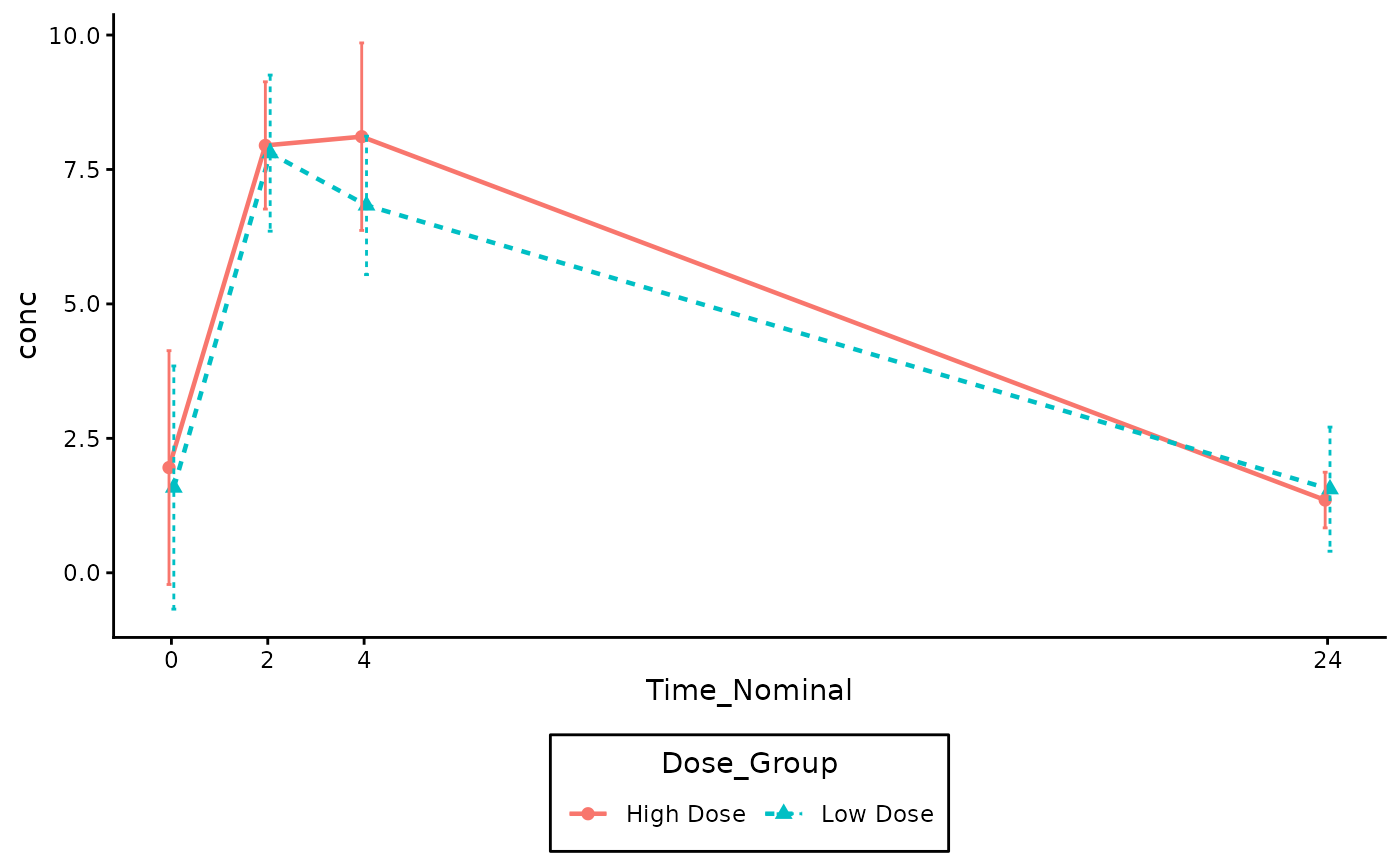
# Linear Scale Example (Baseline 0 is included)
gg_pkc_lineplot(
data = df_pk,
time_var = Time_Nominal,
analyte_var = conc,
group = Dose_Group,
stat = "mean",
variability = "sd",
log_y = FALSE
)
#> ℹ We encourage to supply `time_var` as a factor, since it supports correct
#> decimals formatting in the summary table.
#> Scale for x is already present.
#> Adding another scale for x, which will replace the existing scale.
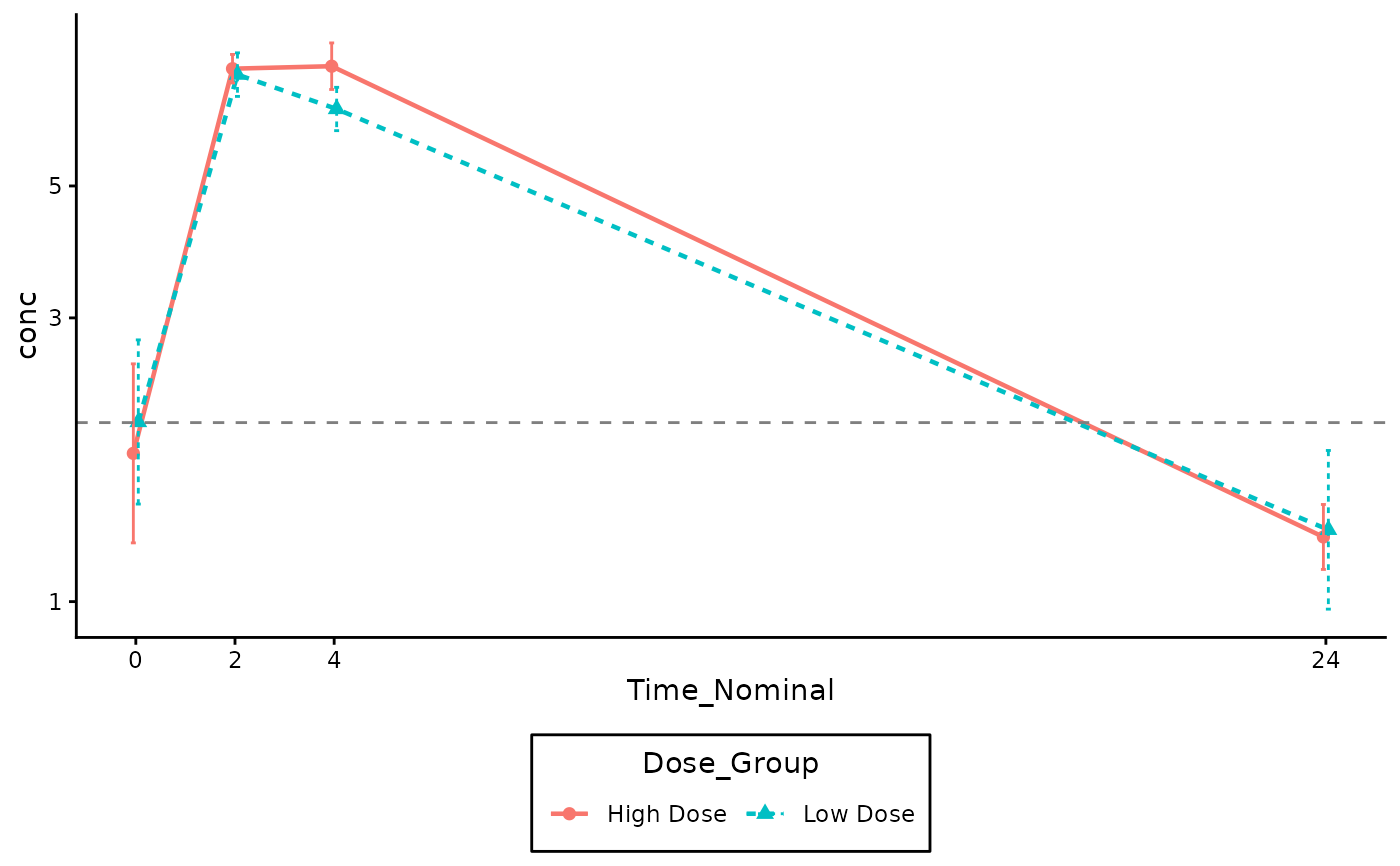
 # Log Scale Example (Filter out 0s first to avoid log(0) warnings)
df_pk |>
dplyr::filter(conc > 0) |>
gg_pkc_lineplot(
time_var = Time_Nominal,
analyte_var = conc,
group = Dose_Group,
stat = "mean",
variability = "se",
log_y = TRUE,
lloq = 2.0
)
#> ℹ We encourage to supply `time_var` as a factor, since it supports correct
#> decimals formatting in the summary table.
#> Scale for x is already present.
#> Adding another scale for x, which will replace the existing scale.
# Log Scale Example (Filter out 0s first to avoid log(0) warnings)
df_pk |>
dplyr::filter(conc > 0) |>
gg_pkc_lineplot(
time_var = Time_Nominal,
analyte_var = conc,
group = Dose_Group,
stat = "mean",
variability = "se",
log_y = TRUE,
lloq = 2.0
)
#> ℹ We encourage to supply `time_var` as a factor, since it supports correct
#> decimals formatting in the summary table.
#> Scale for x is already present.
#> Adding another scale for x, which will replace the existing scale.
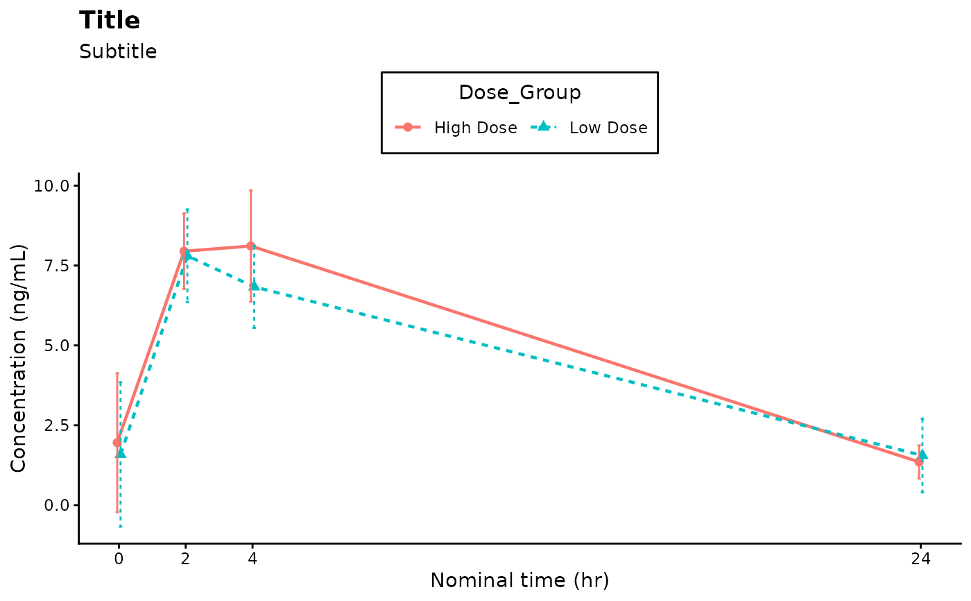
 # Title, subtitle, axes labels and legend position customization
gg_pkc_lineplot(
data = df_pk,
time_var = Time_Nominal,
analyte_var = conc,
group = Dose_Group,
stat = "mean",
variability = "sd",
log_y = FALSE
) +
ggplot2::labs(
x = "Nominal time (hr)",
y = "Concentration (ng/mL)",
title = "Title",
subtitle = "Subtitle"
) +
ggplot2::theme(
legend.position = "top"
)
#> ℹ We encourage to supply `time_var` as a factor, since it supports correct
#> decimals formatting in the summary table.
#> Scale for x is already present.
#> Adding another scale for x, which will replace the existing scale.
# Title, subtitle, axes labels and legend position customization
gg_pkc_lineplot(
data = df_pk,
time_var = Time_Nominal,
analyte_var = conc,
group = Dose_Group,
stat = "mean",
variability = "sd",
log_y = FALSE
) +
ggplot2::labs(
x = "Nominal time (hr)",
y = "Concentration (ng/mL)",
title = "Title",
subtitle = "Subtitle"
) +
ggplot2::theme(
legend.position = "top"
)
#> ℹ We encourage to supply `time_var` as a factor, since it supports correct
#> decimals formatting in the summary table.
#> Scale for x is already present.
#> Adding another scale for x, which will replace the existing scale.