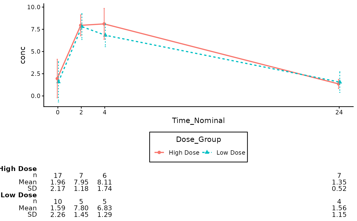
Annotate PK Plot with Summary Table

These functions provide capabilities to annotate Pharmacokinetics plot (gg_pkc_lineplot()) with additional summary statistics table. The annotations are added using the cowplot package for flexible placement.

annotate_pkc_df(
  gg_plt,
  data,
  time_var = NULL,
  analyte_var = NULL,
  group = NULL,
  summary_stats = c("n", "mean", "sd"),
  text_size = 3.5,
  rel_height_plot = 0.75
)

Arguments

gg_plt: (ggplot2)
The PK plot.
data: (data.frame)
The raw or summarized dataset used to generate the table.
time_var, analyte_var, group: (tidy-select)
Optional. If NULL (default), the function automatically extracts these from the gg_plt mapping.
summary_stats: (character)
A vector of statistics to include. Defaults to c("n", "mean", "sd").
text_size: (numeric)
The font size for the table text. Defaults to 3.
rel_height_plot: (numeric)
Relative height of the plot vs the table. Defaults to 0.75.

Examples

# Prepare PK Data using the built-in Theoph dataset
df_pk <- Theoph
df_pk$Time_Nominal <- round(df_pk$Time)
# Filter to specific timepoints to keep the table clean
df_pk <- df_pk[df_pk$Time_Nominal %in% c(0, 2, 4, 8, 24), ]
# Create a mock treatment group based on Dose
df_pk$Dose_Group <- ifelse(df_pk$Dose > 4.5, "High Dose", "Low Dose")

# Create the Base Plot using actual Theoph column names
p_pk <- gg_pkc_lineplot(
  data = df_pk,
  time_var = Time_Nominal,
  analyte_var = conc,
  group = Dose_Group,
  stat = "mean",
  variability = "sd",
  log_y = FALSE
)

# Annotate the Plot (Auto-detects variables from aesthetic mapping)
annotate_pkc_df(
  data = df_pk,
  gg_plt = p_pk
)


# Annotate with specific statistics and explicit variable names
annotate_pkc_df(
  data = df_pk,
  gg_plt = p_pk,
  time_var = "Time_Nominal",
  analyte_var = "conc",
  group = "Dose_Group",
  summary_stats = c("n", "median", "iqr")
)

Arguments

See also

Examples