Introduction

library(bonsaiforest)

In this vignette we are going to show with an example how to use this package.

We are going to consider a data set with time to event data and 10 categorical covariates. These categorical covariates define 25 subgroups. We are interested in estimating the subgroup treatment effect (in this case the subgroup hazard ratio) of each one of these 25 subgroups. Here we will show an example where we only use 2 categorical covariates in order to save run time. To do so we are going to use all the methods available in this package and we are going to compare their results using a forest plot.

Data analysis

As it was mentioned before we are going to use survival data as an example of how to use the package. In our data (that should be of class data.frame) we should have columns with the following variables:

Treatment: factor variable with two levels (the first level represents the control group and the second one the treatment group). It is important to make sure that this variable is a factor and that the levels are in the correct order.
Response: in the case of survival data this should be a numeric variable with the survival time.
Status: in the case of survival data this variable should be present and is a numeric variable with 0 and 1 indicating whether the observation was censored or not.
Categorical variables: factor variables with information about the individuals. The levels of these variables are going to be the subgroups that we are interested in studying.

In our case we have the following structure of the data:

str(example_data)
#> 'data.frame':    1000 obs. of  14 variables:
#>  $ id    : int  1 2 3 4 5 6 7 8 9 10 ...
#>  $ arm   : Factor w/ 2 levels "0","1": 1 1 1 1 2 2 2 2 2 1 ...
#>  $ x_1   : Factor w/ 2 levels "a","b": 2 2 1 1 2 1 1 2 2 1 ...
#>  $ x_2   : Factor w/ 2 levels "a","b": 1 2 1 1 1 2 2 1 2 2 ...
#>  $ x_3   : Factor w/ 2 levels "a","b": 2 1 2 1 2 2 2 1 2 2 ...
#>  $ x_4   : Factor w/ 3 levels "a","b","c": 2 1 3 3 3 3 3 1 3 3 ...
#>  $ x_5   : Factor w/ 4 levels "a","b","c","d": 4 4 1 1 4 1 3 4 4 3 ...
#>  $ x_6   : Factor w/ 2 levels "a","b": 2 1 2 2 2 1 2 2 2 2 ...
#>  $ x_7   : Factor w/ 2 levels "a","b": 2 1 2 2 2 1 1 2 2 2 ...
#>  $ x_8   : Factor w/ 3 levels "a","b","c": 3 2 1 3 3 3 1 1 2 3 ...
#>  $ x_9   : Factor w/ 2 levels "a","b": 2 1 2 2 2 1 1 2 2 2 ...
#>  $ x_10  : Factor w/ 3 levels "a","b","c": 3 3 3 3 3 1 2 2 2 3 ...
#>  $ tt_pfs: num  0.9795 3.4762 1.7947 0.0197 2.2168 ...
#>  $ ev_pfs: num  1 0 1 1 0 0 0 0 0 0 ...

We have that arm is our treatment variable, x_1 to x_10 are the categorical covariates, tt_pfs is the response variable and ev_pfs is the status variable.

Once that we are sure that our data is in the correct format and contains all the necessary variables, we are going to fit the different models in order to obtain the subgroup treatment effects.

Fit Models and Check Summary

Naivepop

Let’s start by fitting the model that will lead to an overall treatment effect estimation.

naivepop_model <- naivepop(
  resp = "tt_pfs",
  trt = "arm",
  data = example_data,
  resptype = "survival",
  status = "ev_pfs"
)

This new naivepop object contains the fitted model, the kind of model that was fitted, the response type of the data and the data.

We can take the summary of this object to obtain the overall treatment effect estimate (in this case the overall hazard ratio).

summary_naivepop <- summary(naivepop_model)
summary_naivepop
#>     arm1 
#> 0.666919

Naive

Now we are going to fit the model to obtain the naive subgroup-specific treatment effects. We have to indicate which categorical variables we want to consider to obtain the subgroup treatment effects. If we add variable x_1 we are going to obtain the subgroup treatment effect of the subgroups x_1a and x_1b. We do the same for x_2.

naive_model <- naive(
  resp = "tt_pfs", trt = "arm",
  subgr = c("x_1", "x_2"),
  data = example_data, resptype = "survival",
  status = "ev_pfs"
)

This naive object contains the fitted models for each one of the subgroups, the main information about the coefficients associated to treatment of these fitted models, the kind of models fitted, the response type and the data.

We can take the summary of this object to obtain the subgroup treatment effects. We can also include a value for the confidence level in order to obtain confidence intervals for these subgroup treatment effect estimates. By default this confidence level is of 95%.

summary_naive <- summary(naive_model, conf = 0.90)
summary_naive
#>   subgroup trt.estimate   trt.low  trt.high
#> 1     x_1a    0.6741880 0.4975147 0.9135999
#> 2     x_1b    0.6645867 0.4936858 0.8946489
#> 3     x_2a    0.7087873 0.5060265 0.9927928
#> 4     x_2b    0.6424496 0.4886396 0.8446746

We can add a forest plot with the estimated treatment effects:

plot(summary_naive)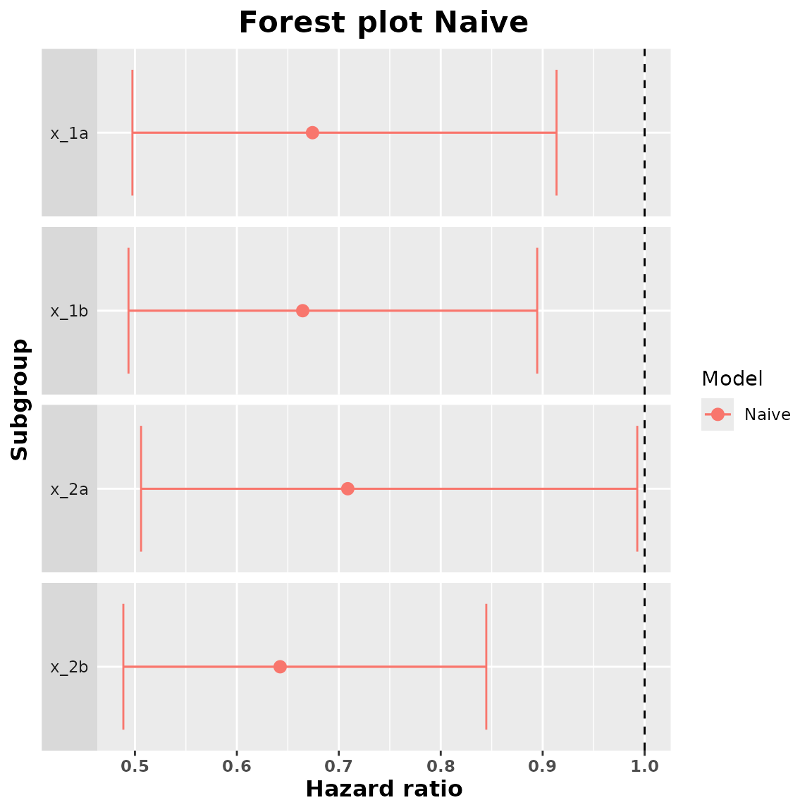

Elastic Net

We are going to fit a model considering an elastic net penalization on the subgroup treatment interaction coefficients. Depending on the value of alpha we are going to have different kinds of penalties. If we put alpha to 0 we consider a ridge penalty and if we put alpha to 1 we consider a lasso penalty. We are going to fit both lasso and ridge.

We have to add the covars argument which indicates which categorical variables we want to include in our model. It is important that all the variables that are in subgr are also in covars. The idea is that we can include many variables but then only find the subgroup treatment effect of some of them.

ridge_model <- elastic_net(
  resp = "tt_pfs", trt = "arm",
  subgr = c("x_1", "x_2"),
  covars = c(
    "x_1", "x_2", "x_3", "x_4", "x_5",
    "x_6", "x_7", "x_8", "x_9", "x_10"
  ),
  data = example_data, resptype = "survival",
  alpha = 0, status = "ev_pfs"
)

lasso_model <- elastic_net(
  resp = "tt_pfs", trt = "arm",
  subgr = c("x_1", "x_2"),
  covars = c(
    "x_1", "x_2", "x_3", "x_4", "x_5",
    "x_6", "x_7", "x_8", "x_9", "x_10"
  ),
  data = example_data, resptype = "survival",
  alpha = 1, status = "ev_pfs"
)

These elastic_net models contain the fitted models, the response type, the data, the value of alpha, the design and the dummy matrices (that are later going to be used to obtain the subgroup treatment effects), the response and status variables and the names of the subgroups.

We are now going to obtain the summary of these fitted objects to find the subgroup hazard ratio estimates.

summary_ridge <- summary(ridge_model)
summary_ridge
#>   subgroup trt.estimate
#> 1     x_1a    0.6502065
#> 2     x_1b    0.6493804
#> 3     x_2a    0.6495783
#> 4     x_2b    0.6501798

summary_lasso <- summary(lasso_model)
summary_lasso
#>   subgroup trt.estimate
#> 1     x_1a    0.6500483
#> 2     x_1b    0.6493824
#> 3     x_2a    0.6493749
#> 4     x_2b    0.6501893

We can obtain a forest plot for each one of these fitted models:

plot(summary_ridge)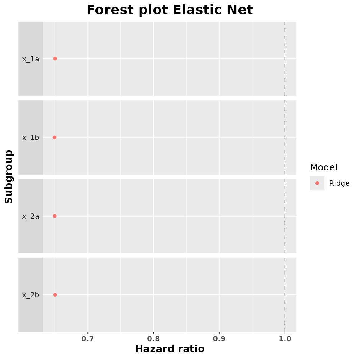

plot(summary_lasso)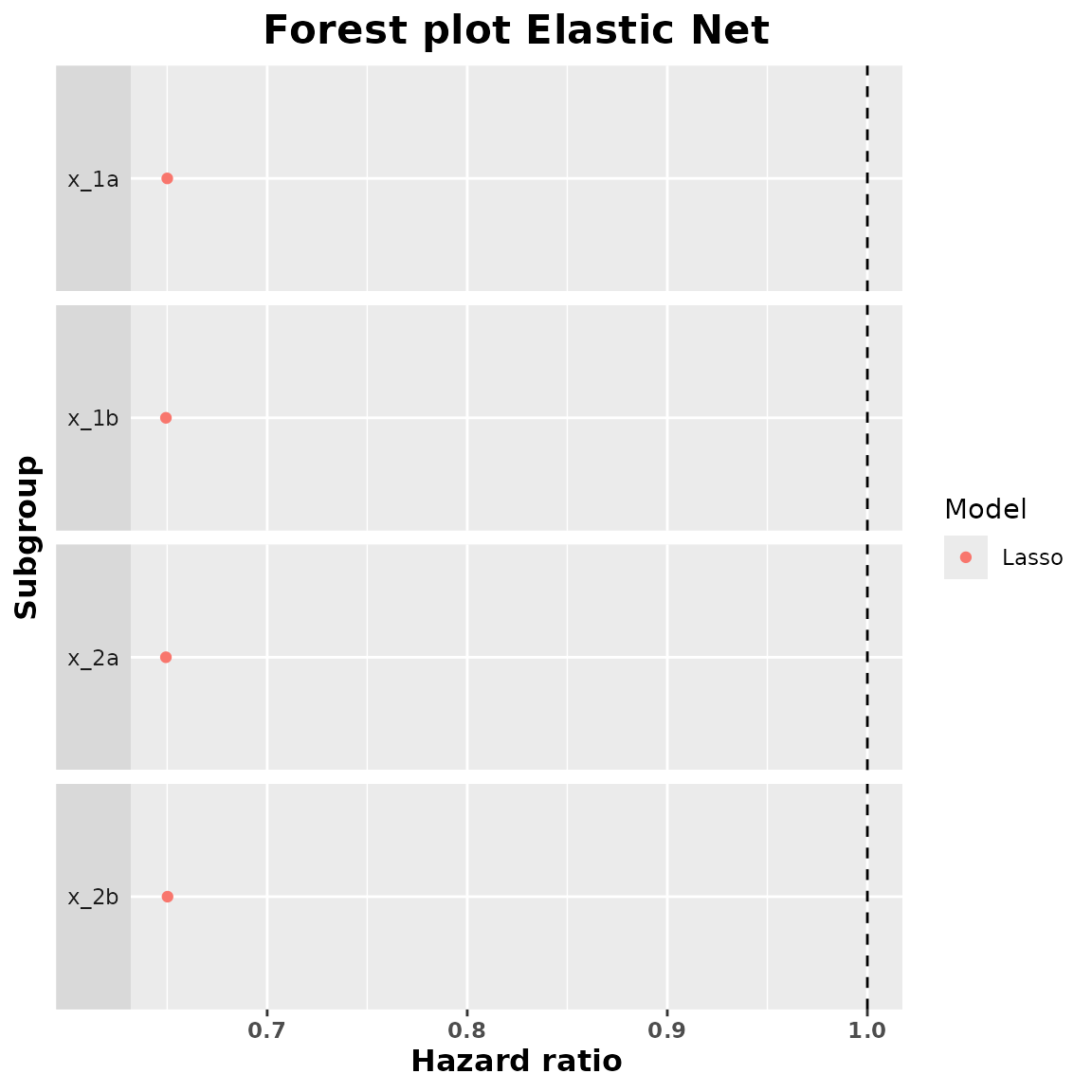

Horseshoe model

We are now going to fit a Bayesian model with a horseshoe prior on the subgroup-treatment interactions. Fitting this kind of models usually takes a bit of time. We can modify some parameters like the number of Markov chains, the number of iterations or the number of warmup iterations (between others). The parameters that we can change are found in the documentation of the brm function from the brms package.

horseshoe_model <- horseshoe(
  resp = "tt_pfs", trt = "arm",
  subgr = c("x_1", "x_2"),
  covars = c(
    "x_1", "x_2", "x_3", "x_4", "x_5",
    "x_6", "x_7", "x_8", "x_9", "x_10"
  ),
  data = example_data,
  resptype = "survival",
  status = "ev_pfs",
  chains = 2,
  seed = 0,
  iter = 1000,
  warmup = 800,
  control = list(adapt_delta = 0.95)
)

Once that the model is fitted we have to check if there are convergence problems. We might get divergent transitions after warmup. In general if there are few divergent transitions (taking into account the total number of iterations) and there are no other problems like high Rhat values we can continue with our analysis.

We can obtain a summary of the posterior distributions of the coefficients of the fitted model:

horseshoe_model$fit
#>  Family: cox 
#>   Links: mu = log 
#> Formula: tt_pfs | cens(1 - ev_pfs) ~ a + b 
#>          a ~ 0 + arm0 + arm1 + x_1b + x_2b + x_3b + x_4b + x_4c + x_5b + x_5c + x_5d + x_6b + x_7b + x_8b + x_8c + x_9b + x_10b + x_10c
#>          b ~ 0 + x_1a_arm + x_1b_arm + x_2a_arm + x_2b_arm + x_3a_arm + x_3b_arm + x_4a_arm + x_4b_arm + x_4c_arm + x_5a_arm + x_5b_arm + x_5c_arm + x_5d_arm + x_6a_arm + x_6b_arm + x_7a_arm + x_7b_arm + x_8a_arm + x_8b_arm + x_8c_arm + x_9a_arm + x_9b_arm + x_10a_arm + x_10b_arm + x_10c_arm
#>    Data: data_model (Number of observations: 1000) 
#>   Draws: 2 chains, each with iter = 1000; warmup = 800; thin = 1;
#>          total post-warmup draws = 400
#> 
#> Regression Coefficients:
#>             Estimate Est.Error l-95% CI u-95% CI Rhat Bulk_ESS Tail_ESS
#> a_arm0         -0.28      0.41    -1.06     0.56 1.04       95      102
#> a_arm1         -0.76      0.54    -1.83     0.29 1.03       97      118
#> a_x_1b         -0.08      0.15    -0.35     0.18 1.02      347      254
#> a_x_2b          0.07      0.13    -0.20     0.32 1.00      531      313
#> a_x_3b         -0.32      0.17    -0.64     0.01 1.01      382      270
#> a_x_4b         -0.27      0.18    -0.64     0.07 1.00      351      282
#> a_x_4c         -0.56      0.19    -0.94    -0.21 1.01      340      270
#> a_x_5b          0.04      0.29    -0.44     0.80 1.00      152       88
#> a_x_5c         -0.13      0.25    -0.55     0.36 1.01      143       93
#> a_x_5d         -0.22      0.23    -0.60     0.30 1.00      137       82
#> a_x_6b          0.20      0.15    -0.12     0.51 1.00      313      262
#> a_x_7b          0.07      0.16    -0.25     0.35 1.00      332      312
#> a_x_8b          0.00      0.20    -0.39     0.37 1.00      289      205
#> a_x_8c         -0.01      0.18    -0.36     0.38 1.00      247      130
#> a_x_9b          0.10      0.20    -0.27     0.45 1.01      303      237
#> a_x_10b         0.18      0.22    -0.24     0.57 1.00      403      365
#> a_x_10c         0.15      0.20    -0.23     0.51 1.00      360      299
#> b_x_1a_arm     -0.00      0.10    -0.20     0.19 1.00      457      316
#> b_x_1b_arm     -0.01      0.11    -0.29     0.20 1.01      473      363
#> b_x_2a_arm      0.01      0.09    -0.16     0.25 1.00      325      281
#> b_x_2b_arm     -0.01      0.10    -0.27     0.18 1.00      435      215
#> b_x_3a_arm     -0.05      0.15    -0.43     0.09 1.02      270      225
#> b_x_3b_arm      0.04      0.13    -0.09     0.43 1.01      325      352
#> b_x_4a_arm     -0.02      0.10    -0.33     0.16 1.00      381      230
#> b_x_4b_arm     -0.02      0.13    -0.35     0.24 1.00      435      367
#> b_x_4c_arm      0.04      0.12    -0.10     0.42 1.01      324      255
#> b_x_5a_arm      0.10      0.25    -0.10     0.92 1.00      130       94
#> b_x_5b_arm     -0.07      0.19    -0.68     0.12 1.01      293      226
#> b_x_5c_arm     -0.03      0.10    -0.33     0.13 1.00      453      377
#> b_x_5d_arm      0.01      0.10    -0.26     0.22 1.00      515      366
#> b_x_6a_arm      0.02      0.11    -0.15     0.30 1.00      412      306
#> b_x_6b_arm     -0.03      0.11    -0.35     0.17 1.00      384      315
#> b_x_7a_arm     -0.07      0.16    -0.58     0.08 1.01      262      223
#> b_x_7b_arm      0.05      0.15    -0.13     0.55 1.01      270      220
#> b_x_8a_arm     -0.03      0.11    -0.41     0.13 1.00      420      335
#> b_x_8b_arm     -0.01      0.11    -0.28     0.19 1.02      336      317
#> b_x_8c_arm      0.04      0.12    -0.10     0.39 1.00      251      249
#> b_x_9a_arm     -0.04      0.14    -0.48     0.12 1.01      226      258
#> b_x_9b_arm      0.04      0.16    -0.19     0.54 1.01      418      308
#> b_x_10a_arm    -0.01      0.10    -0.26     0.22 1.00      440      313
#> b_x_10b_arm     0.00      0.08    -0.18     0.20 1.00      249      364
#> b_x_10c_arm    -0.02      0.10    -0.28     0.14 1.01      515      341
#> 
#> Draws were sampled using sampling(NUTS). For each parameter, Bulk_ESS
#> and Tail_ESS are effective sample size measures, and Rhat is the potential
#> scale reduction factor on split chains (at convergence, Rhat = 1).

Apart from the fitted model this horseshoe object also contains the data, the response, the design and dummy matrices, the kind of response and the subgroup names.

We are now going to call summary of this object to obtain the subgroup hazard ratio estimates. With this summary we are also going to obtain the samples of the approximate posterior distribution of the subgroup hazard ratios. The estimates are just the median of this approximate posterior distribution. We should select a confidence level in order to obtain credible intervals for the subgroup treatment effects. The default confidence level is 95%.

summary_horseshoe <- summary(horseshoe_model, conf = 0.9)
summary_horseshoe
#>   subgroup trt.estimate   trt.low  trt.high
#> 1     x_1a    0.6548058 0.5396242 0.8285532
#> 2     x_1b    0.6555175 0.5250172 0.7978729
#> 3     x_2a    0.6527021 0.5215938 0.8296019
#> 4     x_2b    0.6479122 0.5427992 0.7976948

We can obtain a forest plot with the treatment effect estimates and the credible intervals.

plot(summary_horseshoe)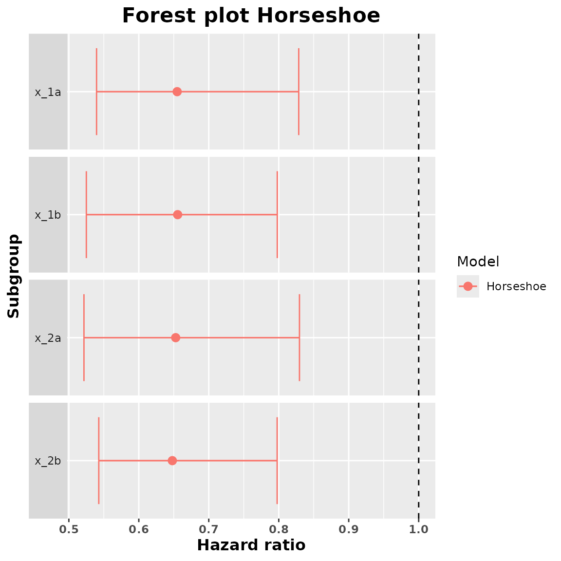

Comparison of the Methods

A last useful thing that we can do is to compare the different treatment effect estimates. For that we are first going to generate a data set with all the estimated hazard ratios and then we are going to plot all of them in a common forest plot.

comparison_data <- compare(naivepop_model, naive_model, ridge_model, lasso_model, horseshoe_model)
comparison_data
#> $data
#>    subgroup trt.estimate   trt.low  trt.high                 model
#> 1      x_1a    0.6741880 0.4693783 0.9683648                 Naive
#> 2      x_1b    0.6645867 0.4663568 0.9470762                 Naive
#> 3      x_2a    0.7087873 0.4743926 1.0589952                 Naive
#> 4      x_2b    0.6424496 0.4636818 0.8901394                 Naive
#> 5      x_1a    0.6502065 0.6502065 0.6502065 Elastic net alpha = 0
#> 6      x_1b    0.6493804 0.6493804 0.6493804 Elastic net alpha = 0
#> 7      x_2a    0.6495783 0.6495783 0.6495783 Elastic net alpha = 0
#> 8      x_2b    0.6501798 0.6501798 0.6501798 Elastic net alpha = 0
#> 9      x_1a    0.6500483 0.6500483 0.6500483 Elastic net alpha = 1
#> 10     x_1b    0.6493824 0.6493824 0.6493824 Elastic net alpha = 1
#> 11     x_2a    0.6493749 0.6493749 0.6493749 Elastic net alpha = 1
#> 12     x_2b    0.6501893 0.6501893 0.6501893 Elastic net alpha = 1
#> 13     x_1a    0.6548058 0.5217772 0.8529706             Horseshoe
#> 14     x_1b    0.6555175 0.5070357 0.8349754             Horseshoe
#> 15     x_2a    0.6527021 0.5113236 0.9065121             Horseshoe
#> 16     x_2b    0.6479122 0.5240480 0.8121235             Horseshoe
#> 
#> $overall_trt
#> [1] 0.666919
#> 
#> $resptype
#> [1] "survival"
#> 
#> attr(,"class")
#> [1] "compare.data"

Now we plot all the estimated subgroup hazard ratios and we add a vertical line indicating the value of the overall hazard ratio.

plot(comparison_data)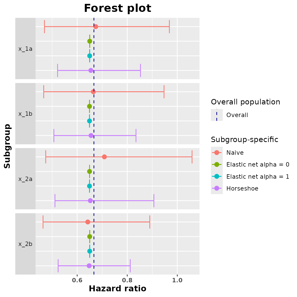

In the case of having survival data the procedure would be analogous but instead of having survival resptype we would have binary. Also the response variable should be a numeric variable with 1 and 0 and there would be no status variable.