![[Stable]](figures/lifecycle-stable.svg)
Usage
g_waterfall(
  height,
  id,
  col_var = NULL,
  col = getOption("ggplot2.discrete.colour"),
  xlab = NULL,
  ylab = NULL,
  col_legend_title = NULL,
  title = NULL
)
Arguments
- height
(
numericvector)
Contains values to be plotted as the waterfall bars- id
(vector)
Contains of IDs used as the x-axis label for the waterfall bars- col_var
(
factor,characterorNULL)
Categorical variable for bar coloring.NULLby default.- col
(
character)
colors.- xlab
(
charactervalue)
x label. Default isID.- ylab
(
charactervalue)
y label. Default isValue.- col_legend_title
(
charactervalue)
Text to be displayed as legend title.- title
(
charactervalue)
Text to be displayed as plot title.
Author
Yuyao Song (songy) yuyao.song@roche.com
Examples
library(nestcolor)
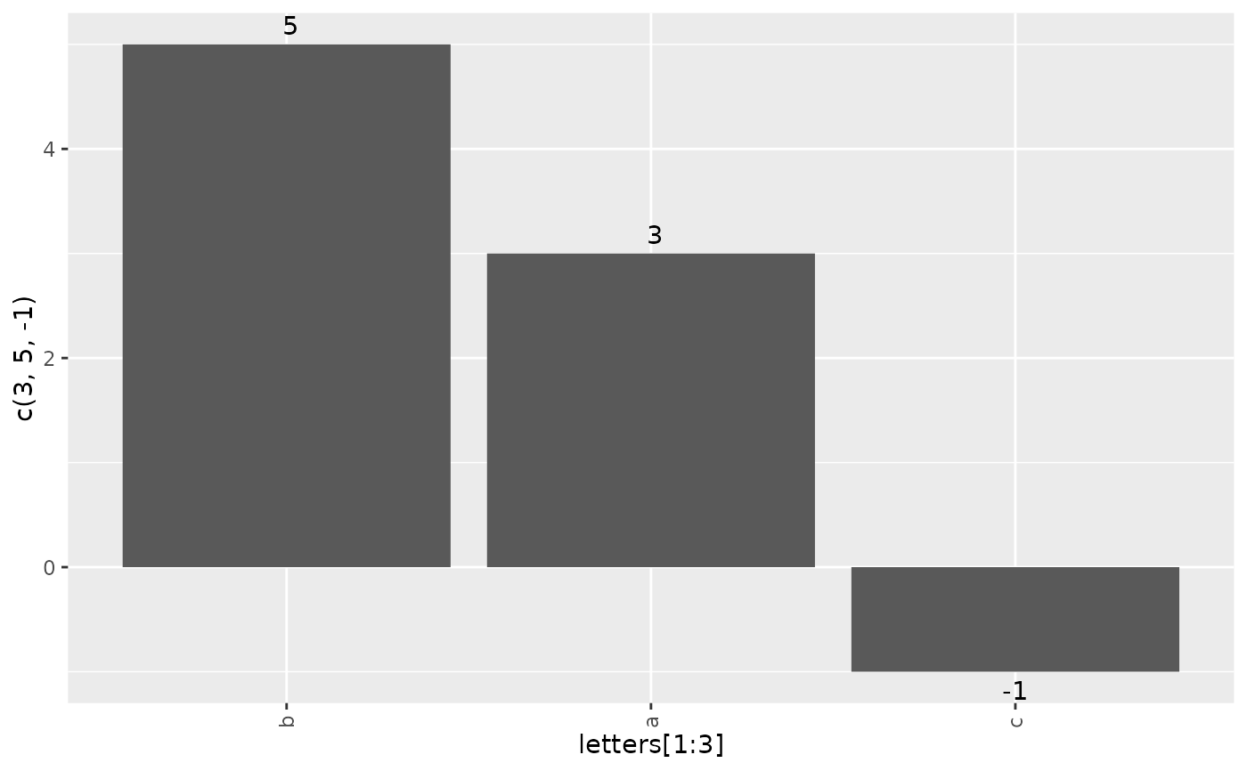
g_waterfall(height = c(3, 5, -1), id = letters[1:3])
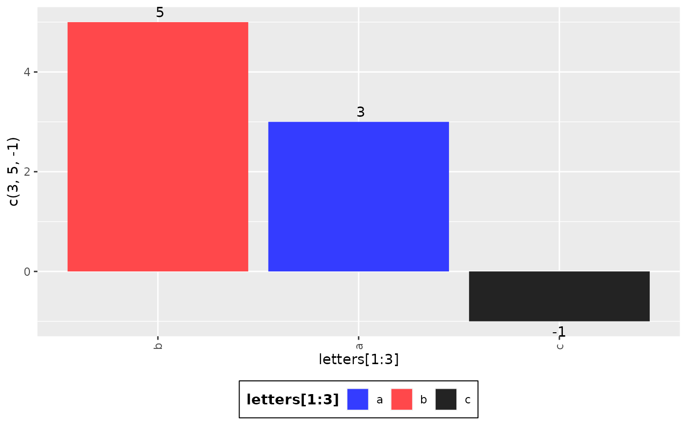
 g_waterfall(
height = c(3, 5, -1),
id = letters[1:3],
col_var = letters[1:3]
)
g_waterfall(
height = c(3, 5, -1),
id = letters[1:3],
col_var = letters[1:3]
)
 library(scda)
library(dplyr)
ADSL <- synthetic_cdisc_data("latest")$adsl
ADSL_f <- ADSL %>%
select(USUBJID, STUDYID, ARM, ARMCD, SEX)
ADRS <- synthetic_cdisc_data("latest")$adrs
ADRS_f <- ADRS %>%
filter(PARAMCD == "OVRINV") %>%
mutate(pchg = rnorm(n(), 10, 50))
ADRS_f <- head(ADRS_f, 30)
ADRS_f <- ADRS_f[!duplicated(ADRS_f$USUBJID), ]
head(ADRS_f)
#> # A tibble: 5 × 67
#> STUDYID USUBJID SUBJID SITEID AGE AGEU SEX RACE ETHNIC COUNTRY DTHFL
#> <chr> <chr> <chr> <chr> <int> <fct> <fct> <fct> <fct> <fct> <fct>
#> 1 AB12345 AB12345-BR… id-105 BRA-1 38 YEARS M BLAC… "HISP… BRA N
#> 2 AB12345 AB12345-BR… id-134 BRA-1 47 YEARS M WHITE "NOT … BRA Y
#> 3 AB12345 AB12345-BR… id-141 BRA-1 35 YEARS F WHITE "NOT … BRA N
#> 4 AB12345 AB12345-BR… id-236 BRA-1 32 YEARS M BLAC… " NOT… BRA N
#> 5 AB12345 AB12345-BR… id-265 BRA-1 25 YEARS M WHITE "NOT … BRA Y
#> # … with 56 more variables: INVID <chr>, INVNAM <chr>, ARM <fct>, ARMCD <fct>,
#> # ACTARM <fct>, ACTARMCD <fct>, TRT01P <fct>, TRT01A <fct>, TRT02P <fct>,
#> # TRT02A <fct>, REGION1 <fct>, STRATA1 <fct>, STRATA2 <fct>, BMRKR1 <dbl>,
#> # BMRKR2 <fct>, ITTFL <fct>, SAFFL <fct>, BMEASIFL <fct>, BEP01FL <fct>,
#> # AEWITHFL <fct>, RANDDT <date>, TRTSDTM <dttm>, TRTEDTM <dttm>,
#> # TRT01SDTM <dttm>, TRT01EDTM <dttm>, TRT02SDTM <dttm>, TRT02EDTM <dttm>,
#> # AP01SDTM <dttm>, AP01EDTM <dttm>, AP02SDTM <dttm>, AP02EDTM <dttm>, …
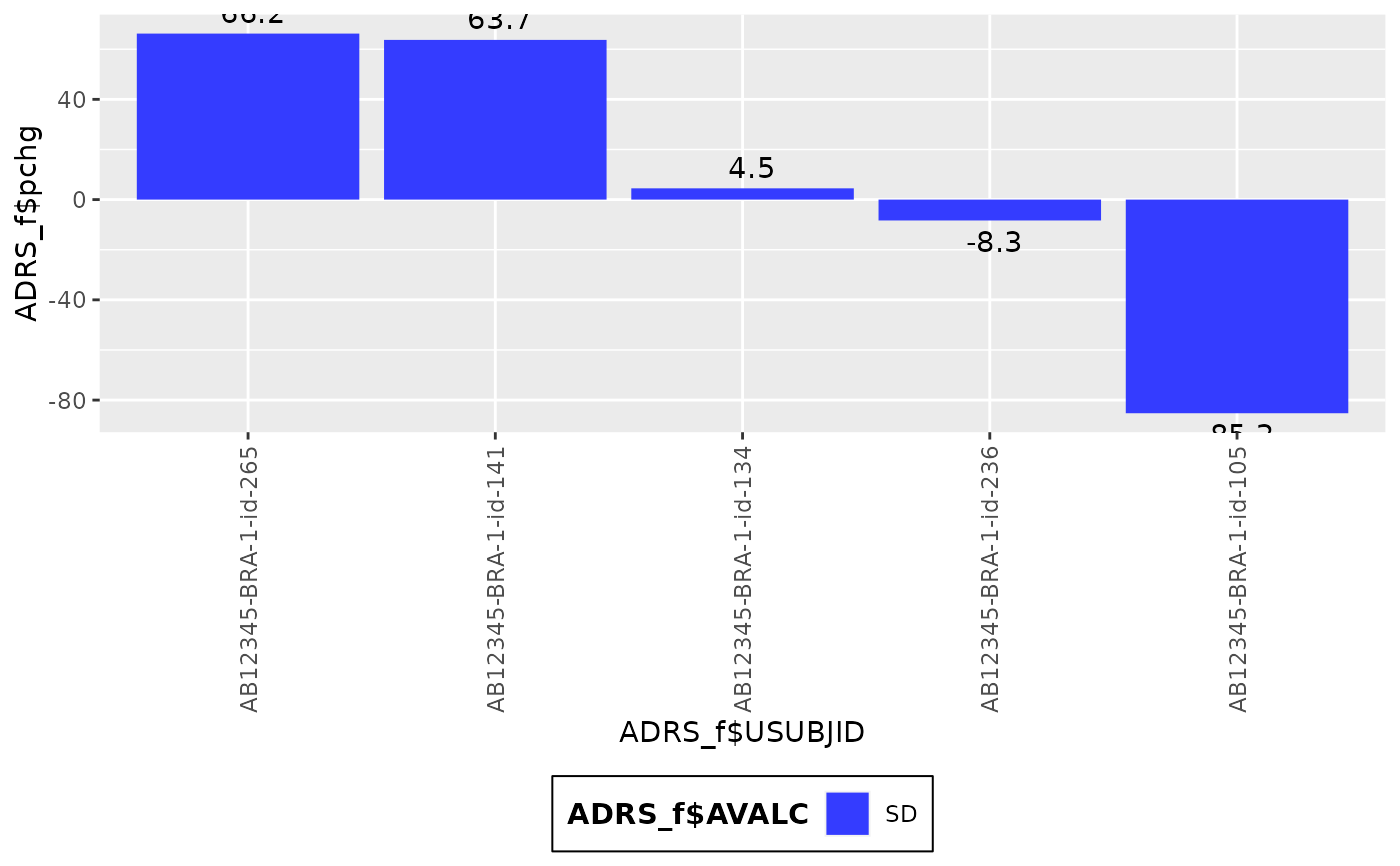
g_waterfall(
height = ADRS_f$pchg,
id = ADRS_f$USUBJID,
col_var = ADRS_f$AVALC
)
library(scda)
library(dplyr)
ADSL <- synthetic_cdisc_data("latest")$adsl
ADSL_f <- ADSL %>%
select(USUBJID, STUDYID, ARM, ARMCD, SEX)
ADRS <- synthetic_cdisc_data("latest")$adrs
ADRS_f <- ADRS %>%
filter(PARAMCD == "OVRINV") %>%
mutate(pchg = rnorm(n(), 10, 50))
ADRS_f <- head(ADRS_f, 30)
ADRS_f <- ADRS_f[!duplicated(ADRS_f$USUBJID), ]
head(ADRS_f)
#> # A tibble: 5 × 67
#> STUDYID USUBJID SUBJID SITEID AGE AGEU SEX RACE ETHNIC COUNTRY DTHFL
#> <chr> <chr> <chr> <chr> <int> <fct> <fct> <fct> <fct> <fct> <fct>
#> 1 AB12345 AB12345-BR… id-105 BRA-1 38 YEARS M BLAC… "HISP… BRA N
#> 2 AB12345 AB12345-BR… id-134 BRA-1 47 YEARS M WHITE "NOT … BRA Y
#> 3 AB12345 AB12345-BR… id-141 BRA-1 35 YEARS F WHITE "NOT … BRA N
#> 4 AB12345 AB12345-BR… id-236 BRA-1 32 YEARS M BLAC… " NOT… BRA N
#> 5 AB12345 AB12345-BR… id-265 BRA-1 25 YEARS M WHITE "NOT … BRA Y
#> # … with 56 more variables: INVID <chr>, INVNAM <chr>, ARM <fct>, ARMCD <fct>,
#> # ACTARM <fct>, ACTARMCD <fct>, TRT01P <fct>, TRT01A <fct>, TRT02P <fct>,
#> # TRT02A <fct>, REGION1 <fct>, STRATA1 <fct>, STRATA2 <fct>, BMRKR1 <dbl>,
#> # BMRKR2 <fct>, ITTFL <fct>, SAFFL <fct>, BMEASIFL <fct>, BEP01FL <fct>,
#> # AEWITHFL <fct>, RANDDT <date>, TRTSDTM <dttm>, TRTEDTM <dttm>,
#> # TRT01SDTM <dttm>, TRT01EDTM <dttm>, TRT02SDTM <dttm>, TRT02EDTM <dttm>,
#> # AP01SDTM <dttm>, AP01EDTM <dttm>, AP02SDTM <dttm>, AP02EDTM <dttm>, …
g_waterfall(
height = ADRS_f$pchg,
id = ADRS_f$USUBJID,
col_var = ADRS_f$AVALC
)
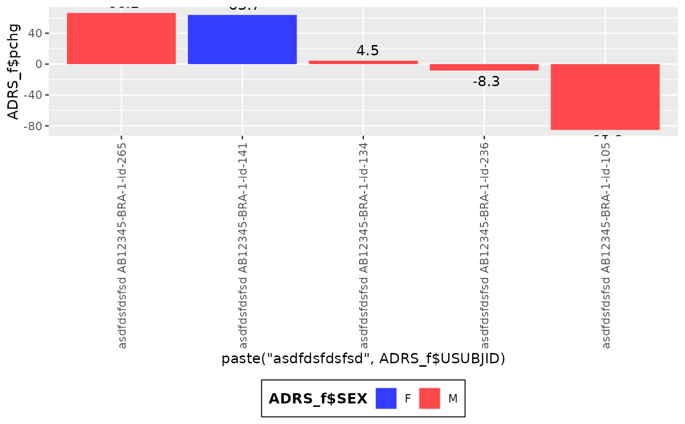
 g_waterfall(
height = ADRS_f$pchg,
id = paste("asdfdsfdsfsd", ADRS_f$USUBJID),
col_var = ADRS_f$SEX
)
g_waterfall(
height = ADRS_f$pchg,
id = paste("asdfdsfdsfsd", ADRS_f$USUBJID),
col_var = ADRS_f$SEX
)
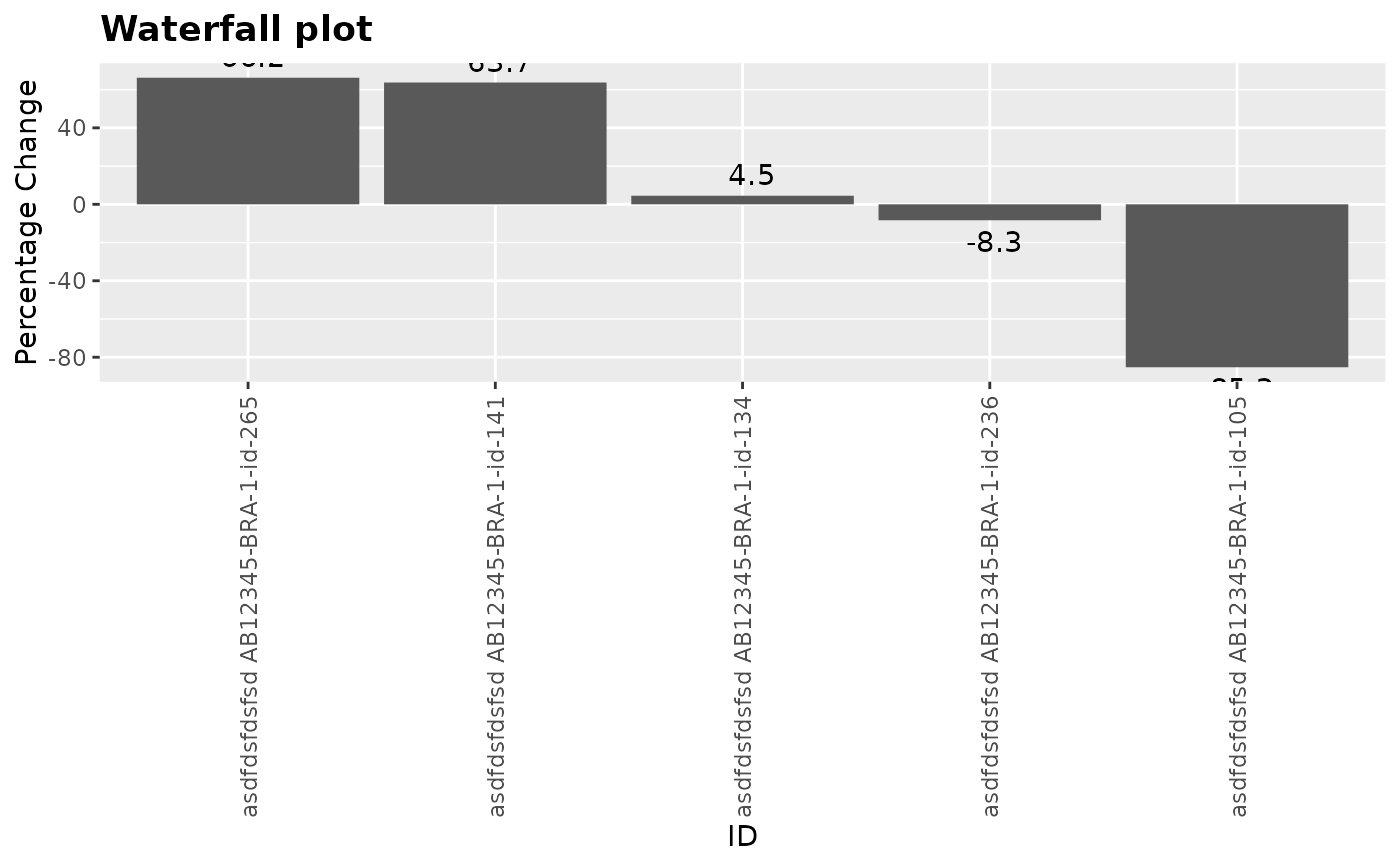
 g_waterfall(
height = ADRS_f$pchg,
id = paste("asdfdsfdsfsd", ADRS_f$USUBJID),
xlab = "ID",
ylab = "Percentage Change",
title = "Waterfall plot"
)
g_waterfall(
height = ADRS_f$pchg,
id = paste("asdfdsfdsfsd", ADRS_f$USUBJID),
xlab = "ID",
ylab = "Percentage Change",
title = "Waterfall plot"
)