![[Stable]](figures/lifecycle-stable.svg)
Based on the STEP results, creates a ggplot graph showing the estimated HR or OR
along the continuous biomarker value subgroups.
Arguments
- df
(
tibble)
result oftidy.step().- use_percentile
(
flag)
whether to use percentiles for the x axis or actual biomarker values.- est
(named
list)colandltysettings for estimate line.- ci_ribbon
(named
listorNULL)fillandalphasettings for the confidence interval ribbon area, orNULLto not plot a CI ribbon.- col
(
character)
colors.- x
(
stepmatrix)
results fromfit_survival_step().- ...
not used here.
Value
The ggplot2 object.
A tibble with one row per STEP subgroup. The estimates and CIs are on the HR or OR scale,
respectively. Additional attributes carry meta data also used for plotting.
Functions
-
tidy(step): Custom Tidy Method for STEP ResultsTidy the STEP results into a
tibbleto format them ready for plotting.
Examples
library(nestcolor)
library(survival)
lung$sex <- factor(lung$sex)
# Survival example.
vars <- list(
time = "time",
event = "status",
arm = "sex",
biomarker = "age"
)
step_matrix <- fit_survival_step(
variables = vars,
data = lung,
control = c(control_coxph(), control_step(num_points = 10, degree = 2))
)
step_data <- broom::tidy(step_matrix)
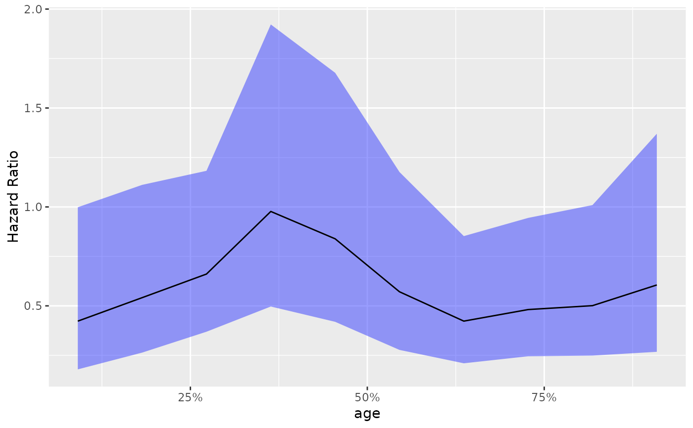
# Default plot.
g_step(step_data)
 # Add the reference 1 horizontal line.
library(ggplot2)
g_step(step_data) +
ggplot2::geom_hline(ggplot2::aes(yintercept = 1), linetype = 2)
# Add the reference 1 horizontal line.
library(ggplot2)
g_step(step_data) +
ggplot2::geom_hline(ggplot2::aes(yintercept = 1), linetype = 2)
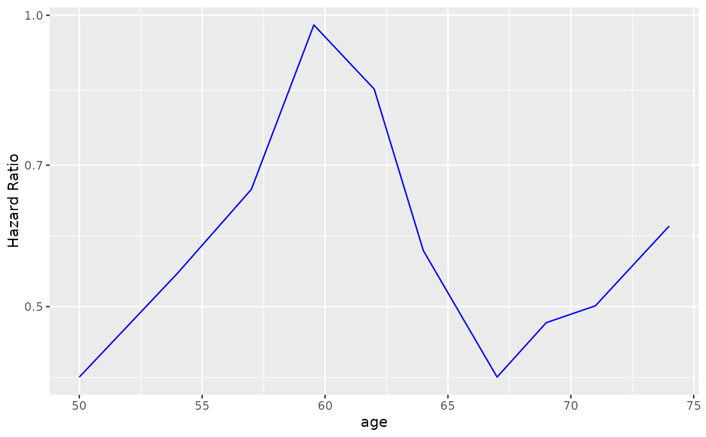
 # Use actual values instead of percentiles, different color for estimate and no CI,
# use log scale for y axis.
g_step(
step_data,
use_percentile = FALSE,
est = list(col = "blue", lty = 1),
ci_ribbon = NULL
) + scale_y_log10()
# Use actual values instead of percentiles, different color for estimate and no CI,
# use log scale for y axis.
g_step(
step_data,
use_percentile = FALSE,
est = list(col = "blue", lty = 1),
ci_ribbon = NULL
) + scale_y_log10()
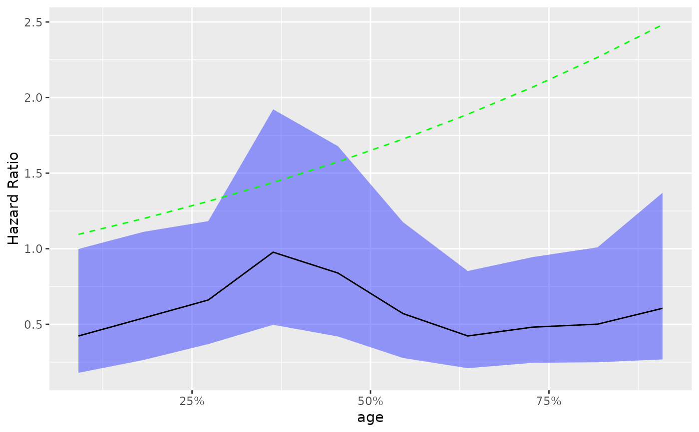
 # Adding another curve based on additional column.
step_data$extra <- exp(step_data$`Percentile Center`)
g_step(step_data) +
ggplot2::geom_line(ggplot2::aes(y = extra), linetype = 2, color = "green")
# Adding another curve based on additional column.
step_data$extra <- exp(step_data$`Percentile Center`)
g_step(step_data) +
ggplot2::geom_line(ggplot2::aes(y = extra), linetype = 2, color = "green")
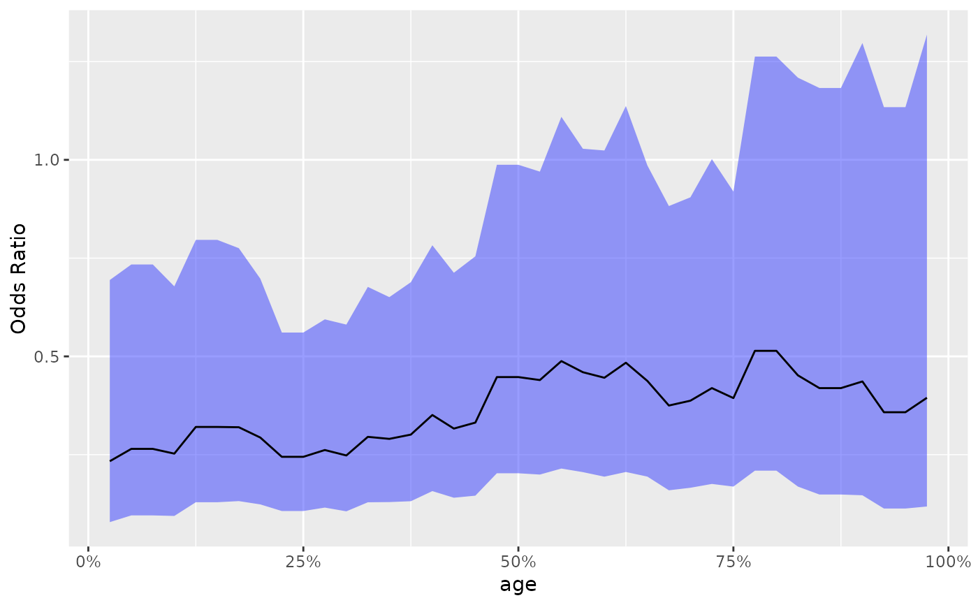
 # Response example.
vars <- list(
response = "status",
arm = "sex",
biomarker = "age"
)
step_matrix <- fit_rsp_step(
variables = vars,
data = lung,
control = c(
control_logistic(response_definition = "I(response == 2)"),
control_step()
)
)
step_data <- broom::tidy(step_matrix)
g_step(step_data)
# Response example.
vars <- list(
response = "status",
arm = "sex",
biomarker = "age"
)
step_matrix <- fit_rsp_step(
variables = vars,
data = lung,
control = c(
control_logistic(response_definition = "I(response == 2)"),
control_step()
)
)
step_data <- broom::tidy(step_matrix)
g_step(step_data)
 library(survival)
lung$sex <- factor(lung$sex)
vars <- list(
time = "time",
event = "status",
arm = "sex",
biomarker = "age"
)
step_matrix <- fit_survival_step(
variables = vars,
data = lung,
control = c(control_coxph(), control_step(num_points = 10, degree = 2))
)
broom::tidy(step_matrix)
#> # A tibble: 10 × 12
#> Percenti…¹ Perce…² Perce…³ Inter…⁴ Inter…⁵ Inter…⁶ n events Hazar…⁷ se
#> * <dbl> <dbl> <dbl> <dbl> <dbl> <dbl> <dbl> <dbl> <dbl> <dbl>
#> 1 0.0909 0 0.341 50 39 59 83 56 0.423 0.438
#> 2 0.182 0 0.432 54 39 61.0 99 68 0.541 0.367
#> 3 0.273 0.0227 0.523 57 43.2 64 122 85 0.661 0.297
#> 4 0.364 0.114 0.614 59.5 50.8 66 117 81 0.977 0.345
#> 5 0.455 0.205 0.705 62 55 68 118 84 0.839 0.354
#> 6 0.545 0.295 0.795 64 58 70 115 82 0.571 0.369
#> 7 0.636 0.386 0.886 67 60 73.2 119 90 0.423 0.358
#> 8 0.727 0.477 0.977 69 63 76.8 116 88 0.481 0.344
#> 9 0.818 0.568 1 71 65 82 100 79 0.501 0.357
#> 10 0.909 0.659 1 74 67 82 85 68 0.606 0.416
#> # … with 2 more variables: ci_lower <dbl>, ci_upper <dbl>, and abbreviated
#> # variable names ¹`Percentile Center`, ²`Percentile Lower`,
#> # ³`Percentile Upper`, ⁴`Interval Center`, ⁵`Interval Lower`,
#> # ⁶`Interval Upper`, ⁷`Hazard Ratio`
library(survival)
lung$sex <- factor(lung$sex)
vars <- list(
time = "time",
event = "status",
arm = "sex",
biomarker = "age"
)
step_matrix <- fit_survival_step(
variables = vars,
data = lung,
control = c(control_coxph(), control_step(num_points = 10, degree = 2))
)
broom::tidy(step_matrix)
#> # A tibble: 10 × 12
#> Percenti…¹ Perce…² Perce…³ Inter…⁴ Inter…⁵ Inter…⁶ n events Hazar…⁷ se
#> * <dbl> <dbl> <dbl> <dbl> <dbl> <dbl> <dbl> <dbl> <dbl> <dbl>
#> 1 0.0909 0 0.341 50 39 59 83 56 0.423 0.438
#> 2 0.182 0 0.432 54 39 61.0 99 68 0.541 0.367
#> 3 0.273 0.0227 0.523 57 43.2 64 122 85 0.661 0.297
#> 4 0.364 0.114 0.614 59.5 50.8 66 117 81 0.977 0.345
#> 5 0.455 0.205 0.705 62 55 68 118 84 0.839 0.354
#> 6 0.545 0.295 0.795 64 58 70 115 82 0.571 0.369
#> 7 0.636 0.386 0.886 67 60 73.2 119 90 0.423 0.358
#> 8 0.727 0.477 0.977 69 63 76.8 116 88 0.481 0.344
#> 9 0.818 0.568 1 71 65 82 100 79 0.501 0.357
#> 10 0.909 0.659 1 74 67 82 85 68 0.606 0.416
#> # … with 2 more variables: ci_lower <dbl>, ci_upper <dbl>, and abbreviated
#> # variable names ¹`Percentile Center`, ²`Percentile Lower`,
#> # ³`Percentile Upper`, ⁴`Interval Center`, ⁵`Interval Lower`,
#> # ⁶`Interval Upper`, ⁷`Hazard Ratio`