Annotate Line Plot with Summary Table

These functions provide capabilities to annotate lineplot (gg_lineplot()) with additional summary statistics table. The annotations are added using the cowplot package for flexible placement.

annotate_lineplot_df(
  gg_plt,
  data,
  x = NULL,
  y = NULL,
  group = NULL,
  summary_stats = c("n", "mean", "sd"),
  digits = NULL,
  rel_height_plot = 0.75
)

Arguments

gg_plt

(ggplot2)
The base line plot generated by gg_lineplot().

data

(data.frame)
The raw data used to generate the statistics.

x, y, group

(string or NULL)
Optional column names as strings. If NULL (default), the function automatically extracts these from the gg_plt mapping.

summary_stats

(character)
Vector of statistics to include. Defaults to c("n", "mean", "sd").

digits

(numeric, list, or formula)
Optional specification for the number of decimal places for the summary statistics. Can be a single integer (e.g., 2), a vector of integers matching the statistics (e.g., c(0, 2, 2)), or a gtsummary style formula. Defaults to NULL (uses gtsummary default auto-formatting).

rel_height_plot

(numeric)
Relative height of the plot vs the table. Defaults to 0.75.

Value

A cowplot object.

See also

gg_lineplot() for related functionalities.

Examples

# 1. Create a mock dataset
set.seed(123)
mock_adlb <- data.frame(
  ARM = rep(c("Treatment A", "Treatment B"), each = 30),
  AVISIT = rep(c(0, 4, 8), 20),
  AVAL = rnorm(60, mean = 10, sd = 2)
)

# 2. Generate the base line plot
p_base <- gg_lineplot(
  data = mock_adlb,
  x = AVISIT,
  y = AVAL,
  group = ARM
)
#> ℹ We encourage to supply `x` as a factor, since it supports correct decimals
#>   formatting in the summary table.

# 3. Annotate with default stats (auto-extracts variables from p_base)
annotate_lineplot_df(gg_plt = p_base, data = mock_adlb)


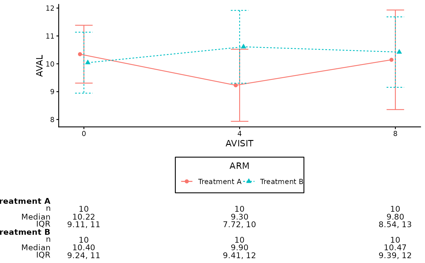
# 4. Annotate with custom statistics and exactly 2 decimal places
annotate_lineplot_df(
  gg_plt = p_base,
  data = mock_adlb,
  summary_stats = c("n", "median", "iqr"),
  digits = c(0, 2, 2)
)